regls.m

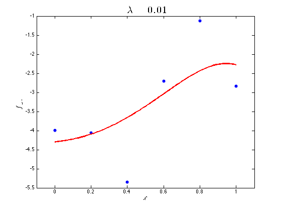
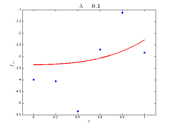
From A First Course in Machine Learning, Chapter 1. Simon Rogers, 31/10/11 [simon.rogers@glasgow.ac.uk] An example of regularised least squares Data is generated from a linear model and then a fifth order polynomial is fitted. The objective (loss) function that is minimisied is

${\cal L} = \lambda \mathbf{w}^T\mathbf{w} + \sum_{n=1}^N (t_n - f(x_n;\mathbf{w}))^2$

Generate the data
Create targets by adding noise
Plot the data
Build up the data so that it has up to fifth order terms
Fit the model with different values of the regularization parameter

Generate the data

x = [0:0.2:1]';
y = 2*x-3;

Create targets by adding noise

noisevar = 3;
t = y + sqrt(noisevar)*randn(size(x));

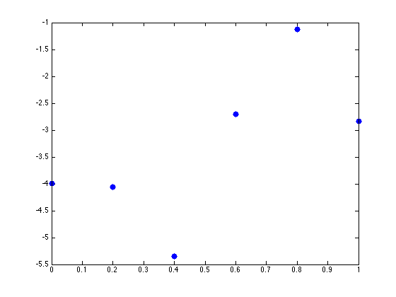
Plot the data

plot(x,t,'b.','markersize',25);

Build up the data so that it has up to fifth order terms

plotX = [0:0.01:1]';
X = [];
plotX = [];
for k = 0:5
    X = [X x.^k];
    plotX =[plotX plotx.^k];
end

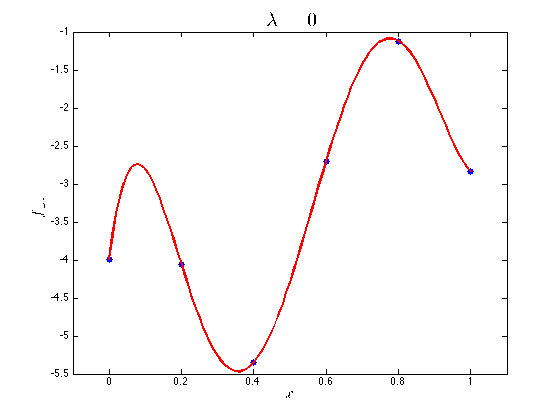
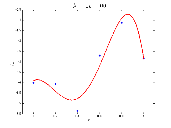
Fit the model with different values of the regularization parameter

$\lambda$

lam = [0 1e-6 1e-2 1e-1];
for l = 1:length(lam)

    lambda = lam(l);
    N = size(x,1);
    w = inv(X'*X + N*lambda*eye(size(X,2)))*X'*t;
    figure(1);hold off
    plot(x,t,'b.','markersize',20);
    hold on
    plot(testX,TestX*w,'r','linewidth',2)
    xlim([-0.1 1.1])
    xlabel('$x$','interpreter','latex','fontsize',15);
    ylabel('$f(x)$','interpreter','latex','fontsize',15);
    ti = sprintf('$\\lambda = %g$',lambda);
    title(ti,'interpreter','latex','fontsize',20)