Contents
w_variation_demo.m
From A First Course in Machine Learning, Chapter 2. Simon Rogers, 01/11/11 [simon.rogers@glasgow.ac.uk] The bias in the estimate of the variance Generate lots of datasets and look at how the average fitted variance agrees with the theoretical value
clear all;close all;
Generate the datasets and fit the parameters
true_w = [-2;3];
Nsizes = [20:20:1000];
for j = 1:length(Nsizes)
    N = Nsizes(j); % Number of objects
    N_data = 10000; % Number of datasets
    x = rand(N,1);
    X = [x.^0 x.^1];
    noisevar = 0.5^2;
    for i = 1:N_data
        t = X*true_w + randn(N,1)*sqrt(noisevar);
        w = inv(X'*X)*X'*t;
        ss = (1/N)*(t'*t - t'*X*w);
        all_ss(j,i) = ss;
    end
end
The expected value of the fitted variance is equal to:
 where
where  is the number of dimensions (2) and
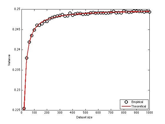
  is the true variance. Plot the average empirical value of the variance against the theoretical expected value as the size of the datasets increases
figure(1);hold off
plot(Nsizes,mean(all_ss,2),'ko','markersize',10,'linewidth',2);
hold on
plot(Nsizes,noisevar*(1-2./Nsizes),'r','linewidth',2);
legend('Empirical','Theoretical','location','Southeast');
xlabel('Dataset size');
ylabel('Variance');