Contents

nonlinlogreg.m

From A First Course in Machine Learning, Chapter 5. Simon Rogers, 01/11/11 [simon.rogers@glasgow.ac.uk] Logistic regression with nonlinear functions

clear all;close all;

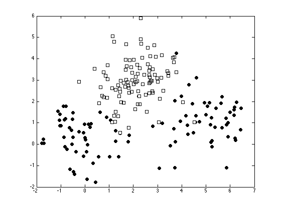
Generate some data

x = [randn(50,2) + repmat([5 1],50,1)];
x = [x; randn(50,2)];
x = [x; randn(100,2) + repmat([2 3],100,1)];
t = [repmat(0,100,1);repmat(1,100,1)];

Plot the data

ma = {'ko','ks'};
fc = {[0 0 0],[1 1 1]};
tv = unique(t);
figure(1); hold off
for i = 1:length(tv)
    pos = find(t==tv(i));
    plot(x(pos,1),x(pos,2),ma{i},'markerfacecolor',fc{i});
    hold on
end

Augment the data with nonlinear terms

X = [x(:,1).^0 x x.^2];

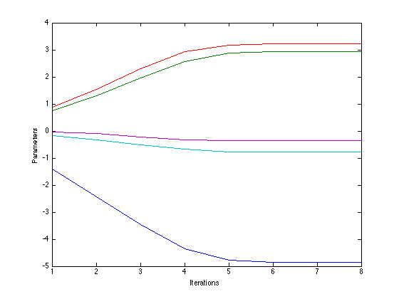
Use the Newton-Raphson MAP solution

%Initisliase the parameters
w = repmat(0,size(X,2),1); % Start at zero
tol = 1e-6; % Stopping tolerance
Nits = 100;
w_all = zeros(Nits,size(X,2)); % Store evolution of w values
ss = 10; % Prior variance on the parameters of w
change = inf;
it = 0;
while change>tol & it<=100
    prob_t = 1./(1+exp(-X*w));
    % Gradient
    grad = -(1/ss)*w' + sum(X.*(repmat(t,1,length(w))-repmat(prob_t,1,length(w))),1);
    % Hessian
    H = -X'*diag(prob_t.*(1-prob_t))*X;
    H = H - (1/ss)*eye(length(w));
    % Update w
    w = w - inv(H)*grad';
    it = it + 1;
    w_all(it,:) = w';
    if it>1
        change = sum((w_all(it,:) - w_all(it-1,:)).^2);
    end
end
w_all(it+1:end,:) = [];

Plot the parameter convergence

figure(1); hold off
plot(w_all);
xlabel('Iterations');
ylabel('Parameters');

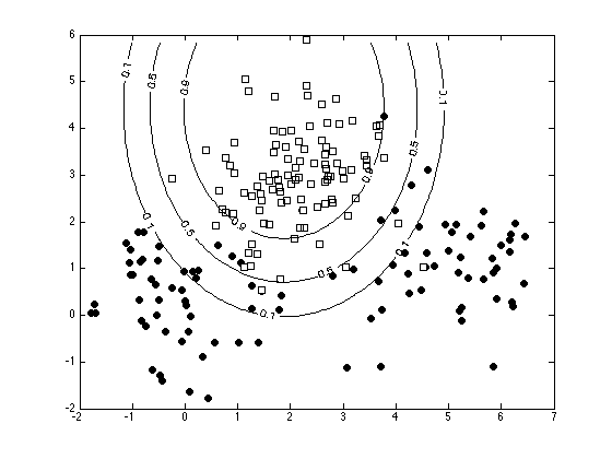
Plot the decision contours

[Xv,Yv] = meshgrid(min(x(:,1)):0.1:max(x(:,1)),min(x(:,2)):0.1:max(x(:,2)));
Pvals = 1./(1 + exp(-(w(1) + w(2).*Xv + w(3).*Yv + w(4).*Xv.^2 + w(5).*Yv.^2)));
figure(1); hold off
for i = 1:length(tv)
    pos = find(t==tv(i));
    plot(x(pos,1),x(pos,2),ma{i},'markerfacecolor',fc{i});
    hold on
end
[c,h] = contour(Xv,Yv,Pvals,[0.1 0.5 0.9],'k');
clabel(c,h)

Published with MATLAB® 7.13