Contents

gpclass.m

Performs binary GP classification with one dimensional data

From A First Course in Machine Learning Simon Rogers, August 2016 [simon.rogers@glasgow.ac.uk]

clear all; close all;

Binary GP classification (1D) using the Laplace approximation

clear all;close all;

% If you don't want the exact data from the book, comment the rng line
% and the two that slightly change x values
rng(100);
N = 10;
x = rand(N,1);
x = sort(x);
x(3) = x(3) + 0.05;
x(10) = x(10) + 0.05;

Set the covariance parameters

gamma = 10;
alpha = 10;

Compute the covariance matrix (training)

for n = 1:N
    for m = 1:N
        C(n,m) = alpha*exp(-gamma*(x(n)-x(m))^2);
    end
end

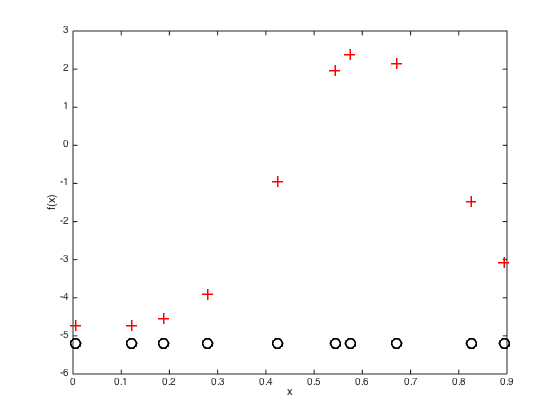
Generative model - Figure 8.18 in book

Change the rng parameter to get different datasets

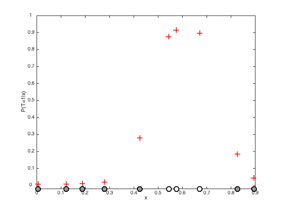
rng(84)
% Sample a function from the GP prior
f = mvnrnd(repmat(0,N,1),C);
figure(1);
hold off;
% Plot the realisations of the function
plot(x,f,'r+','markersize',10,'linewidth',2)
hold on
xlabel('x')
ylabel('f(x)')
yl = ylim;
yl(1) = yl(1) - 0.2;
% Plot the data points along the x axis
plot(x,repmat(yl(1),N,1),'ko','markersize',10,'linewidth',2)

% Convert the function values to probabilities via a sigmoid function
figure(2);hold off
p = 1./(1+exp(-f));
% Plot the probabilities
plot(x,p,'r+','markersize',10,'linewidth',2)
ylim([-0.02 1]);
yl = ylim;
hold on
% Get some random numbers
u = rand(N,1);
t = zeros(N,1);
% Set the target class to 1 if the random value is less than the probability
t(u<=p') = 1;
% Plot the data agin, coloured according to class
pos = find(t==0);
plot(x(pos),repmat(yl(1),length(pos),1),'ko','markersize',10,'linewidth',2,'markerfacecolor',[0.6 0.6 0.6]);
pos = find(t==1);
plot(x(pos),repmat(yl(1),length(pos),1),'ko','markersize',10,'linewidth',2,'markerfacecolor',[1 1 1]);
set(gca,'ytick',[0:0.1:1],'yticklabel',[0:0.1:1])
xlabel('x')
ylabel('P(T=1|x)')

Inference of f

We will start with a point estimate obtained through numerical optimisation

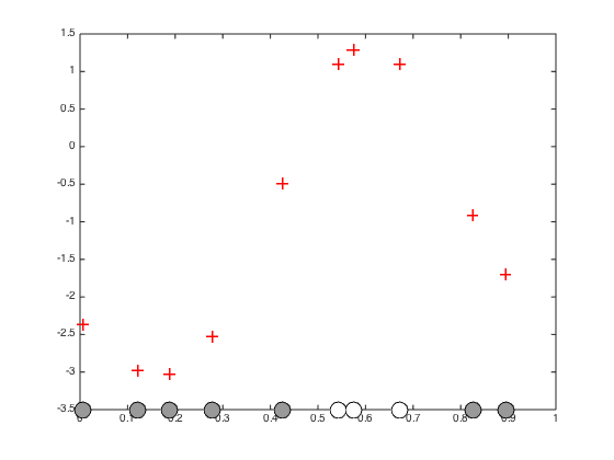
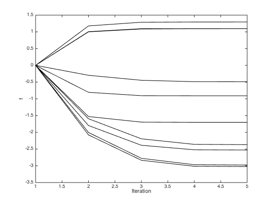
Newton-Rapshon procedure for finding the MAP estimate of f

Initialise f as a vector of zeros

f = zeros(N,1);
% Pre-compute the inverse of C (for efficiency)
invC = inv(C);

% Newton-Raphson procedure (p.300)
max_its = 10;
it = 1;
allf = zeros(max_its,N);
allf(1,:) = f';
while it < max_its
    g = 1./(1+exp(-f));
    gradient = -invC*f + t - g;
    hessian = -invC - diag(g.*(1-g));
    f = f - inv(hessian)*gradient;
    it = it + 1;
    allf(it,:) = f';
end
hessian = -invC - diag(g.*(1-g));

figure();hold off
% Plot the inferred optimised f values
plot(x,f,'r+','markersize',10,'linewidth',2)
hold on
% plot the data
pos = find(t==0);
yl = ylim;
plot(x(pos),repmat(-3.5,length(pos),1),'ko','markersize',15,'markerfacecolor',[0.6 0.6 0.6])
pos = find(t==1);
yl = ylim;
plot(x(pos),repmat(-3.5,length(pos),1),'ko','markersize',15,'markerfacecolor',[1 1 1])
xlim([0 1])

% Plot the evolution of the f values through the optimisation
figure();
plot(allf(1:5,:),'k')
xlabel('Iteration');
ylabel('f');

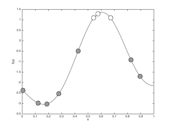
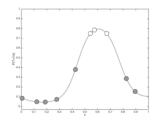
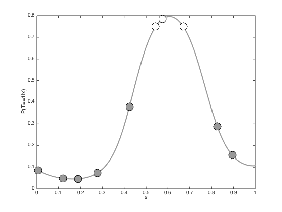
Predictions with the point estimate

Define some test points for vidualisation and compute the test covariance

testx = [0:0.01:1]';
Ntest = length(testx);
% Compute the required covariance functions
for n = 1:N
    for m = 1:Ntest
        R(n,m) = alpha*exp(-gamma*(x(n)-testx(m))^2);
    end
end

for n = 1:Ntest
    for m = 1:Ntest
        Cstar(n,m) = alpha*exp(-gamma*(testx(n) - testx(m))^2);
    end
end

% Compute the latent function at the test points
fs = R'*invC*f;

% Plot the predictive latent function
figure();hold off
plot(testx,fs,'k','color',[0.6 0.6 0.6],'linewidth',2)
hold on
pos = find(t==0);
yl = ylim;
plot(x(pos),f(pos),'ko','markersize',15,'markerfacecolor',[0.6 0.6 0.6])
pos = find(t==1);
plot(x(pos),f(pos),'ko','markersize',15,'markerfacecolor',[1 1 1])
xlabel('x')
ylabel('f(x)')

% Plot the predictive probabilities
figure()
hold off
plot(testx,1./(1+exp(-fs)),'k','linewidth',2,'color',[0.6 0.6 0.6])
hold on
pos = find(t==0);
plot(x(pos),1./(1+exp(-f(pos))),'ko','markersize',15,'markerfacecolor',[0.6 0.6 0.6])
pos = find(t==1);
plot(x(pos),1./(1+exp(-f(pos))),'ko','markersize',15,'markerfacecolor',[1 1 1])
ylim([-0.03 1])
xlabel('x')
ylabel('P(T=1|x)')

Propogating uncertainty through the sigmoid function

In the previous example, we simply pushed the predictive mean through the sigmoid function. We can also account for the predictive variance. Here we do this by generating lots of samples from the latent function, pushing them all through the sigmoid function and then taking the mean

% Comute the predictive variance
predvar = diag(Cstar - R'*invC*R);
% Watch out for really small values
predvar(predvar<1e-6) = 1e-6;

% Generare lots of samples and then average
Nsamples = 10000;
u = randn(Ntest,Nsamples).*repmat(sqrt(predvar),1,Nsamples) + repmat(fs,1,Nsamples);
pavg = mean(1./(1+exp(-u)),2);

% Plot the resulting predictive probabilities
figure();
hold off
plot(testx,pavg,'k','linewidth',2,'color',[0.6 0.6 0.6])
hold on
pos = find(t==0);
plot(x(pos),1./(1+exp(-f(pos))),'ko','markersize',15,'markerfacecolor',[0.6 0.6 0.6])
pos = find(t==1);
plot(x(pos),1./(1+exp(-f(pos))),'ko','markersize',15,'markerfacecolor',[1 1 1])

xlabel('x')
ylabel('P(T==1|x)')

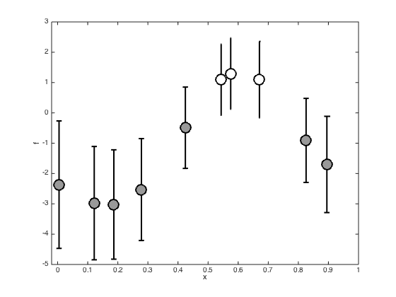
Plot the marginal posterior at the training points

Plot the posterior of the latent variables at the training points (mean plus and minus standard deviation)

figure();
hold off

% Compute the posterior covariance
covf = -inv(hessian);
post_sd = sqrt(diag(covf));
pos = find(t==0);
errorbar(x(pos),f(pos),post_sd(pos),'ko','markersize',15,'markerfacecolor',[0.6 0.6 0.6],'linewidth',2)
hold on
pos = find(t==1);
errorbar(x(pos),f(pos),post_sd(pos),'ko','markersize',15,'markerfacecolor',[1 1 1],'linewidth',2)
xlim([-0.02 1])
xlabel('x')
ylabel('f')

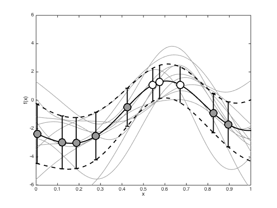
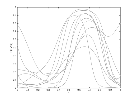
And the test predictions

Add the predictive mean and variance, and some samples to the plots.

% Compute the predictive mean and covariance
pred_mu = R'*invC*f;
pred_cov = Cstar - R'*(C\R) + R'*(C\covf)*invC*R;
pred_cov = pred_cov + 1e-6*eye(Ntest);

figure();
hold off

% Sample some predictive functions and plot them
samps = gausssamp(pred_mu,pred_cov,10);
plot(testx,samps','k','color',[0.6 0.6 0.6])
hold on
% Plot the predictive mean and variance
plot(testx,pred_mu,'k','linewidth',2)
sd = sqrt(diag(pred_cov));
plot(testx,pred_mu + sd,'k--','linewidth',2)
plot(testx,pred_mu - sd,'k--','linewidth',2)

% Plot the values at the data
pos = find(t==0);
errorbar(x(pos),f(pos),post_sd(pos),'ko','markersize',15,'markerfacecolor',[0.6 0.6 0.6],'linewidth',2)
hold on
pos = find(t==1);
errorbar(x(pos),f(pos),post_sd(pos),'ko','markersize',15,'markerfacecolor',[1 1 1],'linewidth',2)
xlim([0 1]);
ylim([-6 6]);

xlabel('x')
ylabel('f(x)')

% Turn each sample into a probability to plot
figure()
hold off
plot(testx,1./(1+exp(-samps')),'k','color',[0.6 0.6 0.6])
ylim([0 1])
xlabel('x')
ylabel('P(T=1|x)')

Published with MATLAB® R2014b