gpclasslaplace.m

Demomnstrates making predictions using the Laplace approximation for GP classification for 1- and 2-D data.

From A First Course in Machine Learning Simon Rogers, August 2016 [simon.rogers@glasgow.ac.uk]

Contents

Full Laplace predictions - 1 dimensional data

We can now look at the full Laplace approximation. Here we sample from the full multivariate Gaussian defined by the Laplace approximation Note that the first cell duplicates lots of things from gpclass.m

Setup things required -- taken from gpclass.m

clear all;close all;

% If you don't want the exact data from the book, comment the rng line
% and the two that slightly change x values
rng(100);
N = 10;
x = rand(N,1);
x = sort(x);
x(3) = x(3) + 0.05;
x(10) = x(10) + 0.05;


% Set the covariance parameters
gamma = 10;
alpha = 10;

% Compute the covariance matrix (training)
for n = 1:N
    for m = 1:N
        C(n,m) = alpha*exp(-gamma*(x(n)-x(m))^2);
    end
end

Generative model - Figure 8.18 in book

Change the rng parameter to get different datasets

rng(84)
% Sample a function from the GP prior
f = mvnrnd(repmat(0,N,1),C);
p = 1./(1+exp(-f));
u = rand(N,1);
t = zeros(N,1);
t(u<=p') = 1;

% Newton-Rapshon procedure for finding the MAP estimate of f
f = zeros(N,1);
invC = inv(C);

% Newton-Raphson procedure (p.300)
max_its = 10;
it = 1;
allf = zeros(max_its,N);
allf(1,:) = f';
while it < max_its
    g = 1./(1+exp(-f));
    gradient = -invC*f + t - g;
    hessian = -invC - diag(g.*(1-g));
    f = f - inv(hessian)*gradient;
    it = it + 1;
    allf(it,:) = f';
end
hessian = -invC - diag(g.*(1-g));


% Predictions with the point estimate
% Define some test points for vidualisation and compute the test covariance
testx = [0:0.01:1]';
Ntest = length(testx);
% Compute the required covariance functions
for n = 1:N
    for m = 1:Ntest
        R(n,m) = alpha*exp(-gamma*(x(n)-testx(m))^2);
    end
end

for n = 1:Ntest
    for m = 1:Ntest
        Cstar(n,m) = alpha*exp(-gamma*(testx(n) - testx(m))^2);
    end
end

% Compute the latent function at the test points
fs = R'*invC*f;

% Compute the posterior covariance
covf = -inv(hessian);

% Compute the predictive mean and covariance
pred_mu = R'*invC*f;
pred_cov = Cstar - R'*(C\R) + R'*(C\covf)*invC*R;
pred_cov = pred_cov + 1e-6*eye(Ntest);

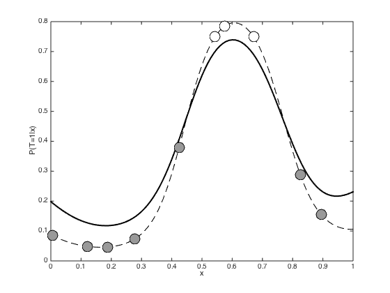
Generate samples from the Laplace approximation and make predictions

figure()
hold off
% Generate 1000 samples from the Laplace approximation
samps = gausssamp(pred_mu,pred_cov,1000);
% Convert into probabilities and compute mean
p = 1./(1+exp(-samps));
p = mean(p,1);
% Plot the Laplace predictions
plot(testx,p,'k','linewidth',2)
hold on
% Plot the point approximation for comparison
plot(testx,1./(1+exp(-fs)),'k--')
pos = find(t==0);
plot(x(pos),1./(1+exp(-f(pos))),'ko','markersize',15,'markerfacecolor',[0.6 0.6 0.6])
pos = find(t==1);
plot(x(pos),1./(1+exp(-f(pos))),'ko','markersize',15,'markerfacecolor',[1 1 1])
xlabel('x')
ylabel('P(T=1|x)')

Laplace approximation for the 2D example

Again, the first cell is setting things up, taken from class2d.m

create some random data and then change the means of the two classes to

seeparate them

rng(2)
x = randn(20,2);
x(1:10,:) = x(1:10,:) - 2;
x(11:end,:) = x(11:end,:) + 2;
t = [repmat(0,10,1);repmat(1,10,1)];


% Set the GP hyperparameters and compute the covariance function

alpha = 10;
gamma = 0.1;
N = size(x,1);
C = zeros(N);
for n = 1:N
    for m = 1:N
        C(n,m) = alpha*exp(-gamma*sum((x(n,:)-x(m,:)).^2));
    end
end


% Newton-raphson procedure to optimise the latent function values
% Initialise all to zero
f = repmat(0,N,1);
allf = [f'];
% Pre-compute the inverse of C
invC = inv(C);
for iteration = 2:6
    g = 1./(1+exp(-f));
    gra = t - g - invC*f;
    H = -diag(g.*(1-g)) - invC;
    f = f - inv(H)*gra;
    allf(iteration,:) = f';
end
H = -diag(g.*(1-g)) - invC;
% Plot the evolution of the f values

% Visualise the predictive function via a large grid of test points
% Create the grid
[X,Y] = meshgrid(-4.5:0.3:4.5,-4.5:0.3:4.5);
testN = prod(size(X));
testX = [reshape(X,testN,1) reshape(Y,testN,1)];
% Create the test covariance function
R = zeros(N,testN);
for n = 1:N
    for m = 1:testN
        R(n,m) = alpha*exp(-gamma*sum((x(n,:) - testX(m,:)).^2));
    end
end

Full Laplace approximation - compute the test covariance

Cstar = zeros(testN);
for n = 1:testN
    for m = 1:testN
        Cstar(n,m) = alpha*exp(-gamma*sum((testX(n,:) - testX(m,:)).^2));
    end
end
covf = -inv(H);
pred_mu = R'*invC*f;
pred_cov = Cstar - R'*(C\R) + R'*(C\covf)*invC*R;
pred_cov = pred_cov + 1e-6*eye(testN);

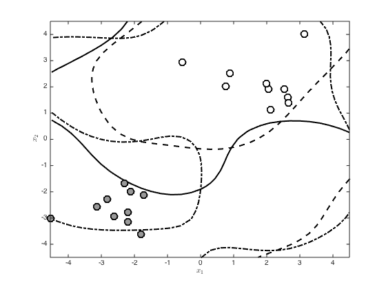
Generate 3 sample functions from the Laplace and plot the resulting decision boundaries

change rng for different samples

rng(11)
figure()
hold off
n_samps = 3;
samps = gausssamp(pred_mu,pred_cov,n_samps);
p = 1./(1+exp(-samps));
styles = {'k','k--','k-.'};
for i = 1:n_samps
    contour(X,Y,reshape(p(i,:),size(X)),[0.5 0.5],styles{i},'linewidth',2)
    hold on
end
pos = find(t==0);
plot(x(pos,1),x(pos,2),'ko','markersize',10,'linewidth',2,'markerfacecolor',[0.6 0.6 0.6])
pos = find(t==1);
plot(x(pos,1),x(pos,2),'ko','markersize',10,'linewidth',2,'markerfacecolor',[1 1 1])
xlabel('$x_1$','interpreter','latex')
ylabel('$x_2$','interpreter','latex')

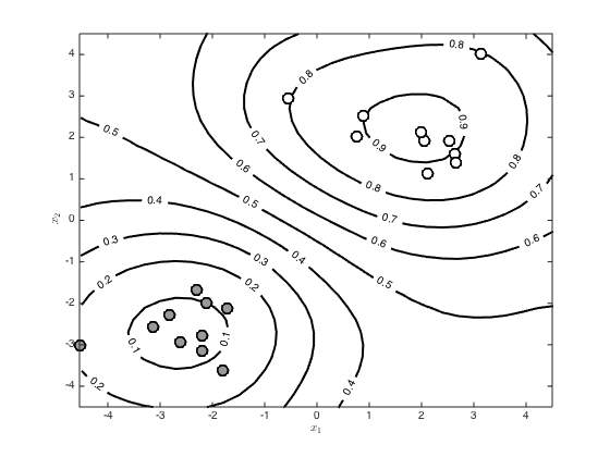
Average over lots of samples from the Laplace

figure()
hold off
n_samps = 1000;
samps = gausssamp(pred_mu,pred_cov,n_samps);
p = 1./(1+exp(-samps));
avgp = mean(p,1);
[c,h] = contour(X,Y,reshape(avgp,size(X)),'k');
clabel(c,h)
set(h,'linewidth',2)
hold on
pos = find(t==0);
plot(x(pos,1),x(pos,2),'ko','markersize',10,'linewidth',2,'markerfacecolor',[0.6 0.6 0.6])
pos = find(t==1);
plot(x(pos,1),x(pos,2),'ko','markersize',10,'linewidth',2,'markerfacecolor',[1 1 1])
xlabel('$x_1$','interpreter','latex')
ylabel('$x_2$','interpreter','latex')

Published with MATLAB® R2014b