Contents

gphyper.m

Performs binary GP classification with two-dimensional data

From A First Course in Machine Learning Simon Rogers, August 2016 [simon.rogers@glasgow.ac.uk]

clear all;close all

Generate the data set, and set the GP hyperparameters

Change rng for different datasets

rng(3)
ss = 0.05;
alpha = 1.0;
gamma = 5.0;
N = 10;
x = rand(N,1);
x = sort(x);

% Dataset hack for nicer visualisation.
x(end) = x(end) - 0.04;

Compute the covariance function

Xdi = (repmat(x,1,length(x)) - repmat(x',length(x),1)).^2;
C = alpha*exp(-gamma*Xdi);

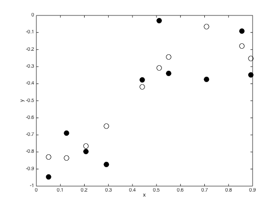
Sample a true latent function

f = gausssamp(repmat(0,N,1),C,1);

% Plot the function
figure()
plot(x,f,'ko','markersize',10);
hold on
f = f';
y = f + randn(N,1).*sqrt(ss);
plot(x,y,'ko','markersize',10,'markerfacecolor','k')
xlabel('x');
ylabel('y');

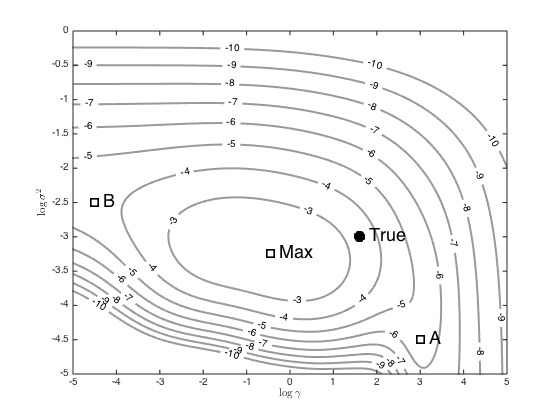
Vary gamma and ss (noise variance) on a grid and see what the marginal likelihood looks like

[G,SS] = meshgrid(-5:0.01:5,-5:0.05:0);
ML = zeros(size(G));
for i = 1:prod(size(G))
    CSS = alpha*exp(-exp(G(i))*Xdi) + exp(SS(i))*eye(N);
    ML(i) = -(N/2)*log(2*pi) - 0.5*log(det(CSS)) - 0.5*y'*inv(CSS)*y;
end

% Contour the results
figure();
hold off
[c,h] = contour(G,SS,ML,[-10:-2],'k','linewidth',2,'color',[0.6 0.6 0.6]);
clabel(c,h);
hold on
plot(log(gamma),log(ss),'ko','markersize',10,'linewidth',2,'markerfacecolor','k')
text(log(gamma)+0.2,log(ss),'True','fontsize',18)

% Plot some points, as used in the book p.313 (these wont make sense if you
% use another dataset)
[r,c] = find(ML == max(ML(:)),1);
other_points = [3 -4.5;-4.5 -2.5;G(r,c) SS(r,c)];
names = {'A','B','Max'};
styles = {'k','k--','b-.'};
for i = 1:length(names)
    plot(other_points(i,1),other_points(i,2),'ks','markersize',10,'linewidth',2)
    text(other_points(i,1)+0.2,other_points(i,2),names{i},'fontsize',18)
end
xlabel('$\log{\gamma}$','interpreter','latex');
ylabel('$\log{\sigma^2}$','interpreter','latex');

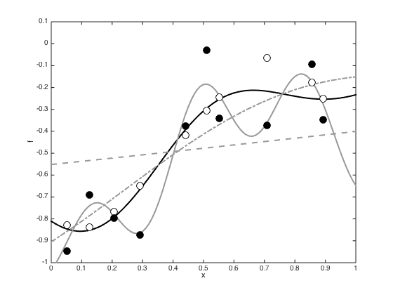
Compute the predictive function with the true covariance parameters, the ones that maximise the marginal likelihood and the ones from points A and B

Define a fine grid of test points

testx = [0:0.01:1]';
testXdi = (repmat(x,1,length(testx)) - repmat(testx',length(x),1)).^2;
testC = alpha*exp(-gamma*testXdi);
% Plot them all
figure();
hold off
testf = testC'*inv(C + ss*eye(N))*y;
plot(testx,testf,'k','linewidth',2)
hold on
for i = 1:length(names)
    otherC = exp(-exp(other_points(i,1))*Xdi);
    othertestC = exp(-exp(other_points(i,1))*testXdi);
    testf = othertestC'*inv(otherC + exp(other_points(i,2))*eye(N))*y;
    plot(testx,testf,styles{i},'linewidth',2,'color',[0.6 0.6 0.6]);
end
plot(x,f,'ko','markersize',10,'markerfacecolor','w');
hold on
plot(x,y,'ko','markersize',10,'markerfacecolor','k')
ylim([-1 0.1])
xlabel('x')
ylabel('f')

Published with MATLAB® R2014b