gpprednoise

gpprednoise.m
Set the kernel parameters
Define x
Create the training covariance matrix
Generate a true function from the GP prior with zero mean
Define the test points - again on a uniform grid
Plot the training data and show the position of the test points
Compute the test covariance
Compute the mean and covariance of the predictions
Plot a smooth predictive function with a one sd window,
Finally, plot some sample functions drawn from the predictive distribution

gpprednoise.m

Performs noisy GP predictions

From A First Course in Machine Learning Simon Rogers, August 2016 [simon.rogers@glasgow.ac.uk]

Note that this is identical to gppred.m with the addition of a diagonal noise component to the training covariance matrix

clear all; close all;

Set the kernel parameters

Try varying these to see the effect

gamma = 0.5;
alpha = 1.0;
sigma_sq = 0.1;

Define x

In this example, we use uniformly spaced x values

x = [-5:2:5];
N = length(x);

Create the training covariance matrix

Firstly for the training data

C = zeros(N);
C = alpha*exp(-gamma*(repmat(x,N,1) - repmat(x',1,N)).^2) + sigma_sq*eye(N);

Generate a true function from the GP prior with zero mean

Define the GP mean

mu = zeros(N,1);
% Sample a function
true_f = mvnrnd(mu,C);

Define the test points - again on a uniform grid

testx = [-4,-2,0,2,4];

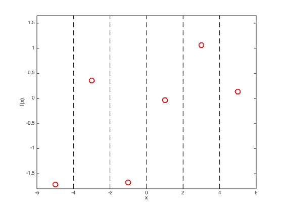
Plot the training data and show the position of the test points

figure();
hold off
plot(x,true_f,'ro','markersize',10,'linewidth',2)
xlabel('x');
ylabel('f(x)');
hold on
% Change the ylimits to make it look nicer
yl = ylim;
yl(1) = 0.9*yl(1);
yl(2) = 1.1*yl(2);
ylim(yl);
xlim([-6,6])
% Draw dashed lines at the test points
for i = testx
    plot([i i],[yl(1) yl(2)],'k--');
end

Compute the test covariance

We need two matrices, $\mathbf{C}^*$ and $\mathbf{R}$ (see page 285)

Ntest = length(testx);
% The train by test matrix
R = alpha*exp(-gamma*(repmat(x',1,Ntest) - repmat(testx,N,1)).^2);
% The test by test matric
Cstar = alpha*exp(-gamma*(repmat(testx,Ntest,1) - repmat(testx',1,Ntest)).^2);

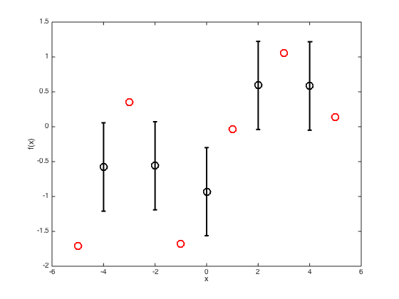
Compute the mean and covariance of the predictions

This uses equation 8.3, p.285

figure()
hold off
% Plot the training data
plot(x,true_f,'ro','markersize',10,'linewidth',2)
% Compute the mean and covariance
pred_mu = R'*inv(C)*true_f';
pred_cov = Cstar - R'*inv(C)*R;
% Extract the standard deviations at the test points (square root of the
% diagonal elements of the covariance matrix)
pred_sd = sqrt(diag(pred_cov));
hold on
% Plot the predictions as error bars
errorbar(testx,pred_mu,pred_sd,'ko','linewidth',2,'markersize',10)
xlim([-6 6]);
xlabel('x')
ylabel('f(x)')

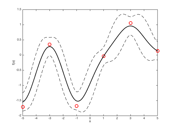
Plot a smooth predictive function with a one sd window,

figure()
hold off
% plot the data
plot(x,true_f,'ro','markersize',10,'linewidth',2)
hold on
% Define a new set of test x values
testx = [-5:0.1:5];
Ntest = length(testx);

% Compute R and Cstar again for the new test points
R = exp(-gamma*(repmat(x',1,Ntest) - repmat(testx,N,1)).^2);
Cstar = exp(-gamma*(repmat(testx,Ntest,1) - repmat(testx',1,Ntest)).^2);

% Compute the predictive mean and covariance
pred_mu = R'*inv(C)*true_f';
pred_cov = Cstar - R'*inv(C)*R;

% Plot the predicted mean and plus and minus one sd
plot(testx,pred_mu,'k','linewidth',2)
plot(testx,pred_mu + sqrt(diag(pred_cov)),'k--')
plot(testx,pred_mu - sqrt(diag(pred_cov)),'k--')

xlabel('x')
ylabel('f(x)')

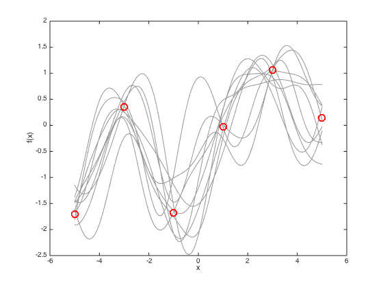
Finally, plot some sample functions drawn from the predictive distribution

figure(4)
hold off
% Plot the data
plot(x,true_f,'ro','markersize',10,'linewidth',2)
hold on
xlim([-6 6])
% Draw 10 samples from the multivariate gaussian
f_samps = mvnrnd(pred_mu,pred_cov,10);
% plot them
plot(testx,f_samps,'k','color',[0.6 0.6 0.6])
% plot the original training data
plot(x,true_f,'ro','markersize',10,'linewidth',2)

xlabel('x')
ylabel('f(x)')

Contents