Contents

convergence.m

Scripts demonstrating issues related to autocorrelation and MCMC convergence

From A First Course in Machine Learning Simon Rogers, August 2016 [simon.rogers@glasgow.ac.uk]

clear all; close all;

Create an object holding some Gaussian contours

clear all;close all;
mu = [1;2];
co = [1 0.8;0.8 2];
[Xv,Yv] = meshgrid([-2:0.1:4],[-1:0.1:5]);
Ci = inv(co);
P = zeros(size(Xv));
for i = 1:size(Xv(:))
    P(i) = - log(2*pi) - 0.5*log(det(co)) - 0.5*([Xv(i)-mu(1) Yv(i)-mu(2)]*Ci*[Xv(i)-mu(1) Yv(i)-mu(2)]');
end
P = exp(P);

Do some MH samples from this Gaussian with multiple chains

figure(); hold off
contour(Xv,Yv,P,'k','linewidth',2,'color',[0.6 0.6 0.6])
hold on

% Vary jump_sig2 to give different levels of convergence
jump_sig2 = 0.4;

% Define the starting points of the chains
start_points = {[-3;1],[5;1],[1.5;5]};
plot_cols = {'ko','r^','gs'};

% Generate 200 samples for each chain and plots the samples
for i = 1:length(start_points)
    accept{i} = 0;
    x = start_points{i};
    S = 2000;
    N = length(x);
    all_samps_mh{i} = zeros(S+1,N);
    all_samps_mh{i}(1,:) = x';
    Ci = inv(co);
    old_log_like = -0.5*(x - mu)'*Ci*(x - mu);
    for s = 1:S
        new_x = x + randn(N,1).*sqrt(jump_sig2);
        new_log_like = -0.5*(new_x - mu)'*Ci*(new_x-mu);
        r = exp(new_log_like - old_log_like);
        if rand <= r
            x = new_x;
            old_log_like = new_log_like;
            accept{i} = accept{i} + 1;
        end
        all_samps_mh{i}(s+1,:) = x';
    end
    plot(all_samps_mh{i}(:,1),all_samps_mh{i}(:,2),plot_cols{i})
    accept{i} = accept{i}/S;
end

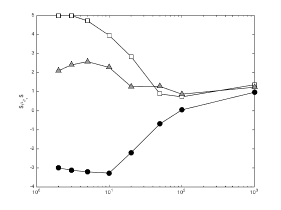
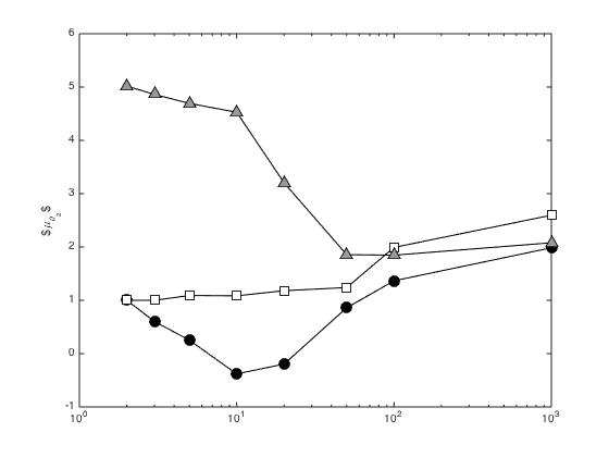
Plot a trace of the sample means at different numbers of samples

Define the samples at which the plots should be made

plot_points = [2,3,5,10,20,50,100,1000];
plot_cols = {'ko','ks','k^'};
fill_cols = {[0 0 0],[1 1 1],[0.6 0.6 0.6]};
fig_no = 1;
for var_no = 1:N
    fig_no = fig_no + 1;
    figure(fig_no);
    hold off
    cum_means{var_no} = [];
    for j = 1:length(start_points)
        for k = 1:length(plot_points)
            cum_means{var_no}(k,j) = mean(all_samps_mh{j}(1:plot_points(k),var_no));
        end
        semilogx(plot_points,cum_means{var_no}(:,j),[plot_cols{j} '-'],'markerfacecolor',fill_cols{j},'markersize',10)
        hold on
        ylabel(sprintf('$\\mu_{\\theta_%g}$',var_no));
    end
end

Compute and plot R_hat

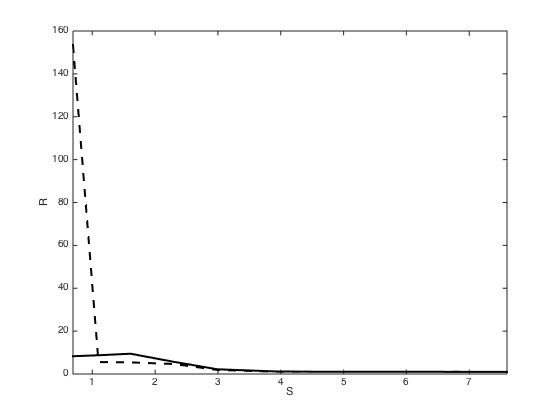
close all
figure();hold off
plot_points = [2,3,5,10,20,50,100,1000,2000];
M = length(start_points);
for par = 1:2
    for i = 1:length(plot_points)
        N = plot_points(i);
        mu_m = [];
        v_m = [];
        for s = 1:length(start_points)
            % Compute R_hat -- see p.333 (a.k.a. The Gooch page)
            mu_m(s) = mean(all_samps_mh{s}(1:N,par));
            v_m(s) = var(all_samps_mh{s}(1:N,par));
            mu_m_mean = mean(mu_m);
            B =(N/(M-1))*sum((mu_m-mu_m_mean).^2);
            W = mean(v_m);
            V = ((N-1)/N)*W + (1/N)*B;
            R(i,par) = sqrt(V/W);
        end
    end
end

plot(log(plot_points),R(:,1),'k','linewidth',2)
hold on
plot(log(plot_points),R(:,2),'k--','linewidth',2)
yl = ylim;
ylim([0 yl(2)])
xlim([log(plot_points(1)) log(plot_points(end))])
xlabel('S')
ylabel('R')

Autocorrelation

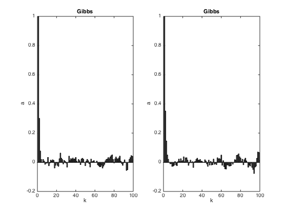
First, so some Gibbs samples for comparison

all_samps_mh{4} = zeros(2000,2);
x = start_points{1};
for i = 1:2000
    % Sample x_1
    mu_1 = mu(1) + (co(1,2)/co(2,2)) * (x(2)-mu(2));
    ss_1 = co(1,1) - co(1,2)^2/co(2,2);
    oldx = x;
    x(1) = randn*sqrt(ss_1) + mu_1;

    % sample x_2
    mu_2 = mu(2) + (co(2,1)/co(1,1)) * (x(1)-mu(1));
    ss_2 = co(2,2) - co(2,1)^2/co(1,1);
    oldx = x;
    x(2) = randn*sqrt(ss_2)+mu_2;

    all_samps_mh{4}(i,:) = x';
end

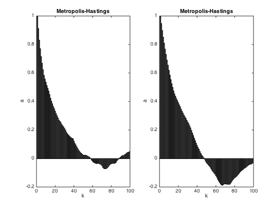
Compute the autocorrelation of the MH and the Gibbs

k_vals = [0:1:100];
s_val = [1,4]; % Plot the AC of the first MH and Gibbs
for start_val = s_val
    figure(start_val)
    ac = zeros(length(k_vals),2);
    for par = 1:2
        temp = all_samps_mh{start_val}(:,par);
        temp = temp - mean(temp);
        N = length(temp);
        ss = var(temp);
        for k = 1:length(k_vals)
            ac(k,par) = sum(temp(1:end-k_vals(k)).*temp(1+k_vals(k):end));
            ac(k,par) = ac(k,par)/(ss*(N-k_vals(k)));
        end
        subplot(1,2,par)
        bar(ac(:,par),'facecolor',[0.6 0.6 0.6])
        xlim([0 100])
        ylim([-0.2 1])
        xlabel('k');
        ylabel('a');
        if start_val == 1
            title('Metropolis-Hastings')
        else
            title('Gibbs')
        end
    end
end

Published with MATLAB® R2014b