You should have already implemented the neural network defined in the instructions for Lab 2, and experimented with the visualisation properties of matlab in order to better understand how a neural network can represent complex mappings.

Begin with a simple single-unit perceptron, as implemented in last week’s lab. We will use a sigmoid response, , where . This neuron will output values in the range 0 to 1. We now want to adjust the parameters of the neuron so that it can best represent the behaviour of a given training set of input, output pairs. It will often not be possible to achieve 100% accuracy, so we need an error or cost function to represent the goodness-of-fit of any particular model given the training data.

We will start with the simple sum-of-squares error function: , which is taking the squared distance between the model output for the nth training input xⁿ and the nth target training output tⁿ. As we have a nonlinear activation function (the sigmoid) we can’t find a closed form solution. As the activation function is differentiable, we can use the derivatives to implement a simple gradient descent approach, such that we try to move in the w-space (by adjusting the parameters of the w-vector) such that the error function decreases. This is an inefficient algorithm but we will use it as a starting point

We start with an initial guess for w and cycle through the training set, adjusting the weights after seeing each pattern, in such a way that we move a small step in the direction of the gradient of the error function.

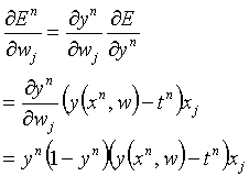
The parameter η is the learning rate, a small positive parameter (we’ll use 0.001 in this case). So we need an expression for the derivative of the error function with respect to the weights.

Note that the last line is true for the sigmoid function but not for the threshold function. Try to prove the derivation of the learning rule yourselves. It involves only standard calculus, as used in school and 1^st year maths. Try to imagine how this would extend to a multi-layer network.

Implement the above code and create a number of training sets to test it (e.g. the logic gates mentioned in last week’s labs, and the data set used last week. Store the value of the error function at the end of each run through the training set. Plot the value of the error function after each training set at the end (after running through the training set say 1000 times - you can experiment with this). At the end, plot the surface of the model at the optimal parameters using the surf command. Try overlaying the training data onto this plot using the plot3() command, and the hold command.

Direct any queries or difficulties to me rod@dcs.gla.ac.uk - I’ll be pleased to help. Note also that frequently asked questions will appear on the NC4 labs web-page, so check there first.

http://www.dcs.gla.ac.uk/~rod/NC4/index.htm

Roderick Murray-Smith