This lab will be ASSESSED (worth 20% of the marks allocated to practical assessment) - make sure that you have completed labs 2 & 3, as they are required to make progress on this one. We are tying together the results from the first two weeks, training a multi-layer perceptron, testing it and writing a short report. This should be handed in at the lab in week 16.

You should have already implemented the neural network defined in the instructions for Lab 2, and experimented with the visualisation properties of matlab in order to better understand how a neural network can represent complex mappings. Lab 3 introduced learning in the single neuron case. We shall now extend this to a full multi-layer perceptron.

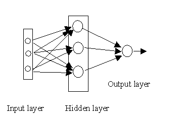
In this example we will build a multi-layer perceptron which has one output y, and n inputs x, with h hidden neurons. Last week’s lab on learning in a single neuron gives us the learning algorithm for the weights from the hidden neurons to the output y – we just repeat everything, but instead of the inputs x (as used last week), the inputs are the activations of the last layer of hidden units, g. How do we determine the weights of layers further back in the network? These layers could also be viewed as single perceptrons but we have no target training values to give them – we don’t know how to assign credit in learning. For networks with differentiable activation functions (such as the sigmoid function we are using) the outputs become differentiable functions of both the input variables and the weights and biases. Error functions such as the sum-of-squares error function are also differentiable, so we can evaluate the derivatives of the error with respect to the weights. These derivatives can be used to find weight values which minimise the error function (we learn something useful) by using either gradient descent, or as we will later examine a more powerful optimisation technique. This is often called the error back-propagation technique.

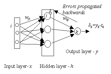
In lab 2 you created MATLAB code for the forward propagation stage. This calculates the activation of the hidden neurons and output neurons for a given set of inputs.We now need to implement the backward propagation stage, where the mismatch between the calculated output and the desired output associated with each input-output training pair (x,t) is fed back through the network. Note that the error E_n only depends on the weight w_ji (from unit i to unit j) via the summed input a_j to neuron j, so we can use the chain rule for partial derivatives to give

Introduce the notation:

where the δ’s are referred to as errors. The derivative of the error by the weights (they way we want to move if we want to learn something) can then be written

which is the same general form as for single layer networks. The δ is the error associated with the output neuron j, while the second part is related to the input to that from neuron i. In order to evaluate the derivatives of the network we need to calculate δ_j for each hidden and output neuron in the network, and apply the above equation.

For output neurons,

For the hidden neurons we again use the chain rule for partial derivatives,

,

where the sum runs over all units k to which neuron j sends connections w_kj. The units labelled k could be hidden or output units. For sigmoid neurons and sum of squares error functions we therefore get:

For output neurons,

For the hidden neurons we obtain the back-propagation formula which shows how the errors are propagated backwards through the network from output to earlier hidden layers. The h are the outputs of the hidden neurons.

,

Once the errors have been back-propagated, we have the derivatives and we can use this to adjust the weights. For the output layer we have

and for the hidden layer

As in Lab 3, the weight adjustment could then be

The figure below might help give some insight into the back-propagation algorithm:

Implement the above in MATLAB and create a number of training sets to test it (e.g. the logic gates mentioned in last week’s labs, and the ballet/rugby data set used last week.

Using either Word or Latex (or similar word processors), write a short report on your experiment, including plots (integrated into the text – not just attached to the end). If you want to convert a picture into .eps format for use with latex or Word, you can use print –depsc filename.eps

This will be marked out of 20, so each point is 1% of your practical assessment.

From the worksheet for Lab 2. Implement the single neuron with a threshold and a sigmoid function in Matlab, and include line and surface plots of the response for different settings of w and w₀, and for different ranges of input, in one and two-dimensional input spaces. Explain in words the effect of the w and w₀ parameters. Give example neurons with weight vectors w and offsets w₀ which simulate AND, OR and NOT functions for two inputs. Is it possible to implement XOR? (Think of the truth tables supplying the test data, and ignore outputs for inputs other than 0 & 1.)

From Lab 3. Implement the MATLAB code for learning in a single neuron case with a sigmoid function and create a number of training sets to test it (e.g. the logic gates mentioned lab 2, and the data set used last week). Store the value of the error function at the end of each run through the training set. Plot the value of the error function after each training set at the end (after running through the training set say 1000 times - you can experiment with this) and include this in the report. At the end, plot the surface of the model at the optimal parameters using the surf() command or the contour command. Try overlaying the training data onto this plot using the plot3() command for 3D surface plots, or the plot() command for 2D plots, and the hold on command. Include your MATLAB code in the report.

Implement the multi-layer perceptron as in lab 2, and the back-propagation algorithm described in this week’s lab. Apply this to the rugby/ballet data, and document the results in a similar manner to Part II above. Include your MATLAB code.

Direct any queries or difficulties to me rod@dcs.gla.ac.uk - I’ll be pleased to help. Note also that frequently asked questions will appear on the NC4 labs web-page, so check there first.

http://www.dcs.gla.ac.uk/~rod/NC4/index.htm

Roderick Murray-Smith