Contents

olynmpbayes.m

From A First Course in Machine Learning, Chapter 2. Simon Rogers, 01/11/11 [simon.rogers@glasgow.ac.uk] Bayesian treatment of Olympic data

clear all;close all;

Load Olympic data

load ../data/olympics

x = male100(:,1);
t = male100(:,2);

% Rescale x for numerical stability
x = x - x(1);
x = x./4;

Define the prior

$p(\mathbf{w}) = {\cal N}(\mu_0,\Sigma_0)

mu0 = [0;0];
si0 = [100 0;0 5];
ss = 2; % Vary this to see the effect on the posterior samples

Draw some functions from the prior

path(path,'../utilities');
w = gausssamp(mu0,si0,10);
X = [x.^0 x.^1];
% Plot the data and the function
figure(1);hold off
plot(x,t,'bo','markersize',10);
hold on
xl = xlim;
yl = ylim;
for i = 1:10
    plot(x,X*w(i,:)','r');
end
xlim(xl);
ylim(yl);

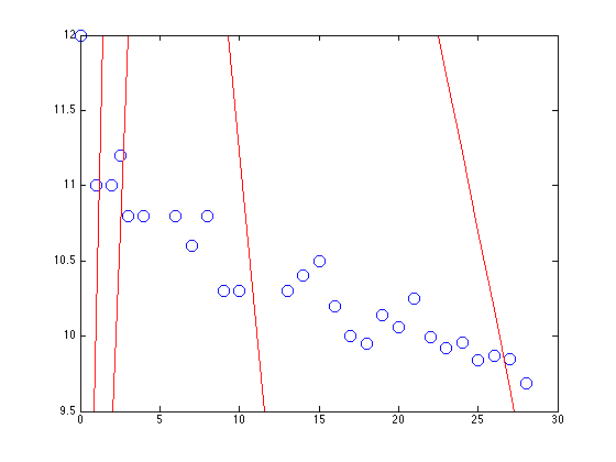
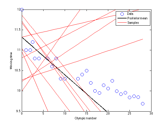
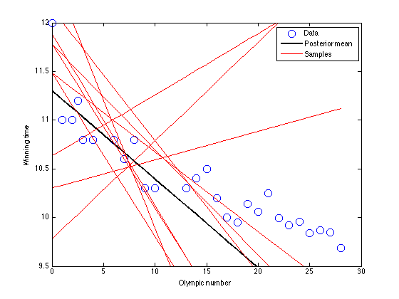
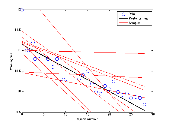
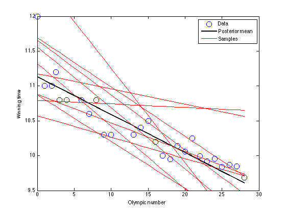
Add the data 3 points at a time

dord = [3:3:length(x)];
for i = 1:length(dord)

    Xsub = X(1:dord(i),:);
    tsub = t(1:dord(i));
    siw = inv((1/ss)*Xsub'*Xsub + inv(si0));
    muw = siw*((1/ss)*Xsub'*tsub + inv(si0)*mu0);
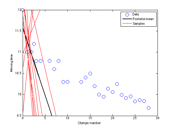
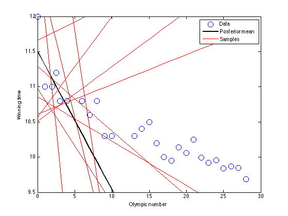
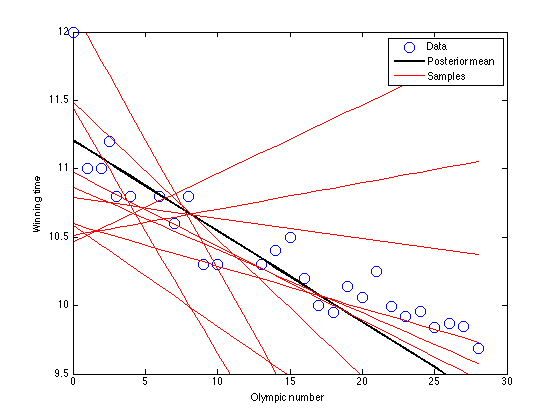
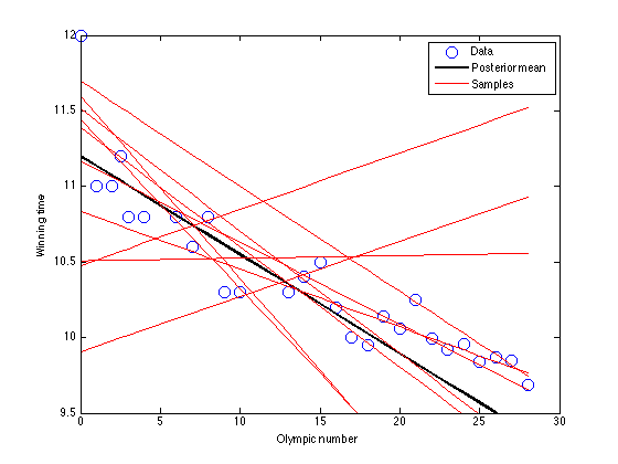
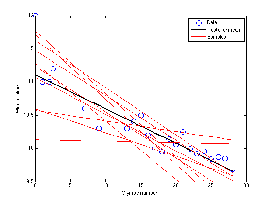
    figure(1);hold off
    plot(x,t,'bo','markersize',10);
    hold on
    xl = xlim;
    yl = ylim;
    plot(x,X*muw,'k','linewidth',2);
    wsamp = gausssamp(muw,siw,10);
    for j = 1:10
        plot(x,X*wsamp(j,:)','r');
    end
    xlim(xl);
    ylim(yl);
    legend('Data','Posterior mean','Samples')
    xlabel('Olympic number');
    ylabel('Winning time');

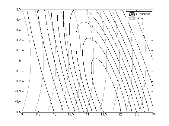
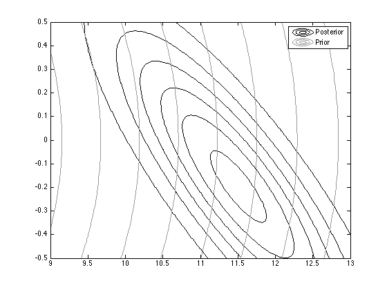
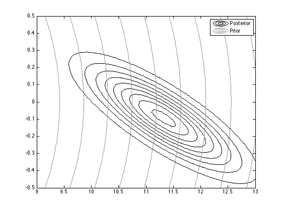
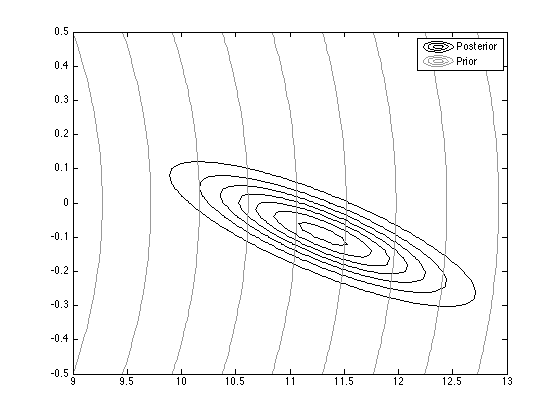
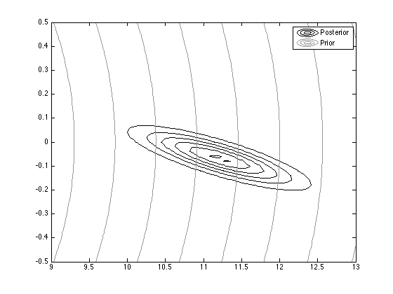
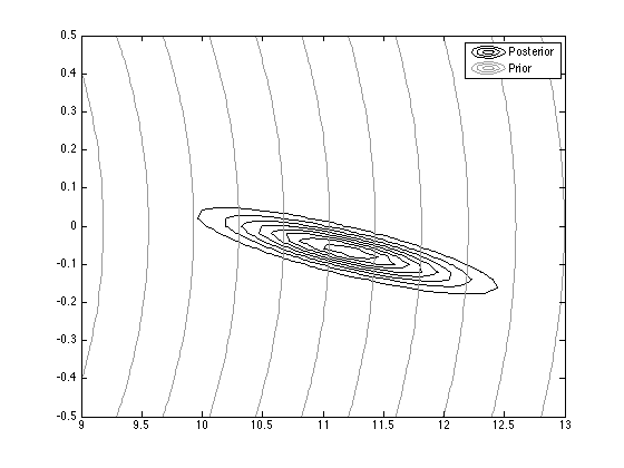
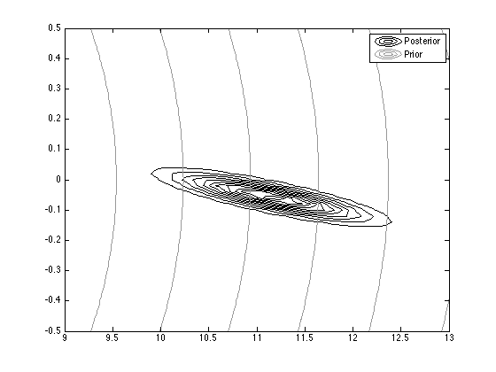
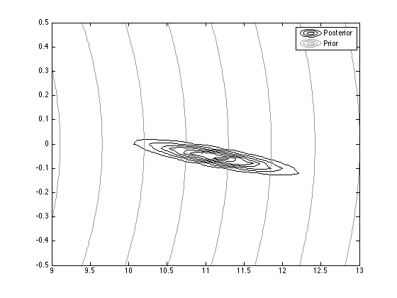
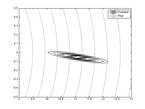
    % Contour plot the prior and posterior

    [Xv,Yv] = meshgrid(9:0.02:13,-0.5:0.02:0.5);

    const = (1/sqrt(2*pi))^2;
    const_prior = const./sqrt(det(si0));
    const = const./sqrt(det(siw));

    temp = [Xv(:)-muw(1) Yv(:)-muw(2)];
    temp_prior = [Xv(:)-mu0(1) Yv(:)-mu0(2)];
    pdfv = const*exp(-0.5*diag(temp*inv(siw)*temp'));
    pdfv = reshape(pdfv,size(Xv));
    pdfv_prior = const*exp(-0.5*diag(temp_prior*inv(si0)*temp_prior'));
    pdfv_prior = reshape(pdfv_prior,size(Xv));
    figure(2);hold off
    contour(Xv,Yv,pdfv,'color','k');
    figure(2);hold on
    contour(Xv,Yv,pdfv_prior,'color',[0.6 0.6 0.6]);
    legend('Posterior','Prior');

end

Published with MATLAB® 7.12