Contents

loglap.m

From A First Course in Machine Learning, Chapter 4. Simon Rogers, 01/11/11 [simon.rogers@glasgow.ac.uk] The Laplace approximation for logistic regression

clear all;close all;

Load the classification data

load ../data/logregdata

Find the mode and the Hessian (see logmap.m)

w = repmat(0,2,1); % Start at zero
tol = 1e-6; % Stopping tolerance
Nits = 100;
w_all = zeros(Nits,2); % Store evolution of w values
ss = 10; % Prior variance on the parameters of w
change = inf;
it = 0;
while change>tol | it<=100
    prob_t = 1./(1+exp(-X*w));
    % Gradient
    grad = -(1/ss)*w' + sum(X.*(repmat(t,1,length(w))-repmat(prob_t,1,length(w))),1);
    % Hessian
    H = -X'*diag(prob_t.*(1-prob_t))*X;
    H = H - (1/ss)*eye(length(w));
    % Update w
    w = w - inv(H)*grad';
    it = it + 1;
    w_all(it,:) = w';
    if it>1
        change = sum((w_all(it,:) - w_all(it-1,:)).^2);
    end
end
w_all(it+1:end,:) = [];

Set the Laplace approximation

muw = w;
siw = inv(-H);

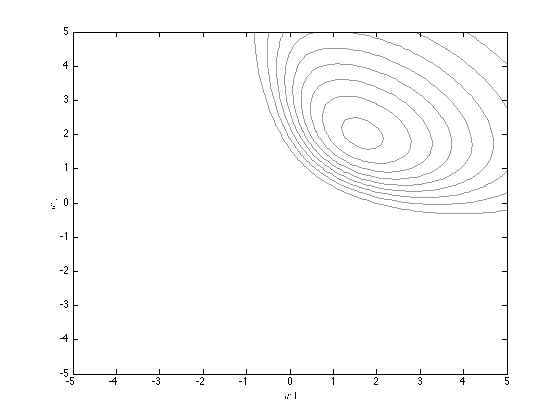
Plot the true posterior (note that we can only get this in unnormalised form)

[w1,w2] = meshgrid(-5:0.1:5,-5:0.1:5);
logprior = -0.5*log(2*pi) - 0.5*log(ss) - (1/(2*ss))*w1.^2;
logprior = logprior + (-0.5*log(2*pi) - 0.5*log(ss) - (1/(2*ss))*w2.^2);
prob_t = 1./(1+exp(-[w1(:) w2(:)]*X'));
loglike = sum(log(prob_t).*repmat(t',prod(size(w1)),1),2);
loglike = loglike + sum(log(1-prob_t).*repmat(1-t',prod(size(w1)),1),2);
logpost = logprior + reshape(loglike,size(w1));
contour(w1,w2,exp(logpost),'k','color',[0.6 0.6 0.6])
xlabel('$w1$','interpreter','latex');
ylabel('$w2$','interpreter','latex');

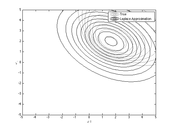
Overlay the approximation

temp = [w1(:)-muw(1) w2(:)-muw(2)];
D = 2; % Working in 2 dimensions
logconst = -(D/2)*log(2*pi) - 0.5*log(det(siw));
log_truepost = logconst - diag(0.5*temp*inv(siw)*temp');
hold on
contour(w1,w2,reshape(exp(log_truepost),size(w1)),'k');
legend('True','Laplace Approximation');

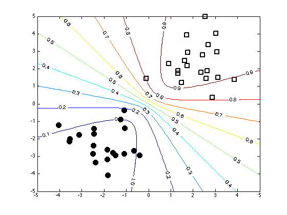
Plot the decision contours

% Create an x grid
[Xv,Yv] = meshgrid(-5:0.1:5,-5:0.1:5);

% Generate samples from the approximate posterior
path(path,'../utilities');
Nsamps = 1000;
w_samps = gausssamp(muw,siw,Nsamps);

% Compute the probabilities over the grid by averaging over the samples
Probs = zeros(size(Xv));
for i = 1:Nsamps
    Probs = Probs + 1./(1 + exp(-(w_samps(i,1)*Xv + w_samps(i,2)*Yv)));
end
Probs = Probs./Nsamps;
figure(1);hold off
plot(X(1:20,1),X(1:20,2),'ko','markersize',10,'markerfacecolor','k')
hold on
plot(X(21:40,1),X(21:40,2),'ks','markersize',10,'linewidth',2)
[cs,h] = contour(Xv,Yv,Probs);
clabel(cs,h);

Published with MATLAB® 7.12