Contents

plotcc.m

From A First Course in Machine Learning, Chapter 5. Simon Rogers, 01/11/11 [simon.rogers@glasgow.ac.uk] Computing and plotting class-conditional densities for a Bayes classifier

clear all;close all;

Load the data

load ../data/bc_data

% Plot the data
cl = unique(t);
col = {'ko','kd','ks'}
fcol = {[1 0 0],[0 1 0],[0 0 1]};
figure(1);
hold off
for c = 1:length(cl)
    pos = find(t==cl(c));
    plot(X(pos,1),X(pos,2),col{c},...
        'markersize',10,'linewidth',2,...
        'markerfacecolor',fcol{c});
    hold on
end
xlim([-3 7])
ylim([-6 6])

col = 

    'ko'    'kd'    'ks'

Fit class-conditional Gaussians for each class

Using the Naive (independence) assumption

for c = 1:length(cl)
    pos = find(t==cl(c));
    % Find the means
    class_mean(c,:) = mean(X(pos,:));
    class_var(c,:) = var(X(pos,:),1);
end

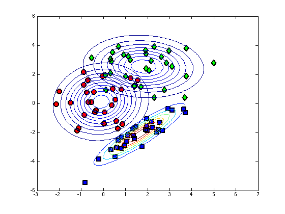
Plot the contours

[Xv,Yv] = meshgrid(-3:0.1:7,-6:0.1:6);
for c = 1:length(cl)
    temp = [Xv(:)-class_mean(c,1) Yv(:)-class_mean(c,2)];
    tempc = diag(class_var(c,:));
    const = -log(2*pi) - log(det(tempc));
    Probs = exp(const - 0.5*diag(temp*inv(tempc)*temp'));
    contour(Xv,Yv,reshape(Probs,size(Xv)));
end

Repeat without Naive assumption

class_var = [];
for c = 1:length(cl)
    pos = find(t==cl(c));
    % Find the means
    class_mean(c,:) = mean(X(pos,:));
    class_var(:,:,c) = cov(X(pos,:),1);
end

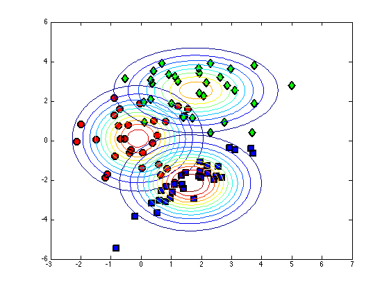
Plot the contours

figure(1);
hold off
for c = 1:length(cl)
    pos = find(t==cl(c));
    plot(X(pos,1),X(pos,2),col{c},...
        'markersize',10,'linewidth',2,...
        'markerfacecolor',fcol{c});
    hold on
end
xlim([-3 7])
ylim([-6 6])
[Xv,Yv] = meshgrid(-3:0.1:7,-6:0.1:6);
for c = 1:length(cl)
    temp = [Xv(:)-class_mean(c,1) Yv(:)-class_mean(c,2)];
    tempc = class_var(:,:,c);
    const = -log(2*pi) - log(det(tempc));
    Probs = exp(const - 0.5*diag(temp*inv(tempc)*temp'));
    contour(Xv,Yv,reshape(Probs,size(Xv)));
end

Published with MATLAB® 7.12