Contents

svmsoft.m

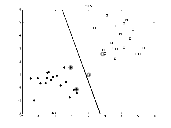
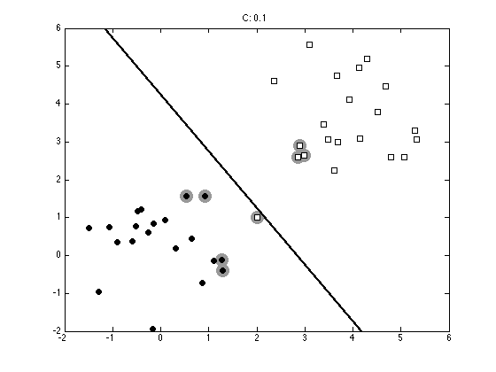
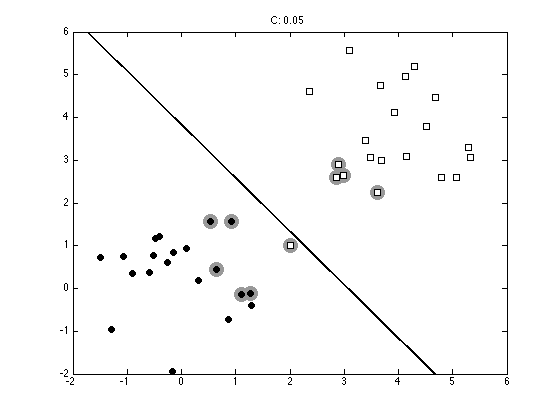
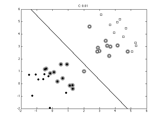
From A First Course in Machine Learning, Chapter 4. Simon Rogers, 01/11/11 [simon.rogers@glasgow.ac.uk] Soft margin SVM

clear all;close all;

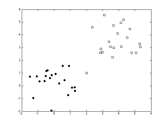
Generate the data

x = [randn(20,2);randn(20,2)+4];
t = [repmat(-1,20,1);repmat(1,20,1)];
% Add a bad point
x = [x;2 1];
t = [t;1];

Plot the data

ma = {'ko','ks'};
fc = {[0 0 0],[1 1 1]};
tv = unique(t);
figure(1); hold off
for i = 1:length(tv)
    pos = find(t==tv(i));
    plot(x(pos,1),x(pos,2),ma{i},'markerfacecolor',fc{i});
    hold on
end

Setup the optimisation problem

N = size(x,1);
K = x*x';
H = (t*t').*K + 1e-5*eye(N);
f = repmat(1,N,1);
A = [];b = [];
LB = repmat(0,N,1); UB = repmat(inf,N,1);
Aeq = t';beq = 0;


warning off

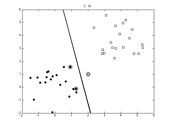
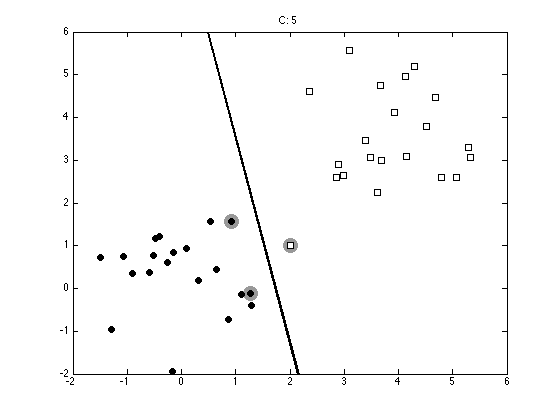
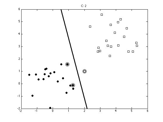
Loop over various values of the margin parameter

Cvals = [10 5 2 1 0.5 0.1 0.05 0.01];
for cv = 1:length(Cvals);

    UB = repmat(Cvals(cv),N,1);
    % Following line runs the SVM
    alpha = quadprog(H,-f,A,b,Aeq,beq,LB,UB);
    % Compute the bias
    fout = sum(repmat(alpha.*t,1,N).*K,1)';
    pos = find(alpha>1e-6);
    bias = mean(t(pos)-fout(pos));

Optimization terminated.

Optimization terminated.

Optimization terminated.

Optimization terminated.

Optimization terminated.

Optimization terminated.

Optimization terminated.

Optimization terminated.

Plot the data, decision boundary and Support vectors

    figure(1);hold off
    pos = find(alpha>1e-6);
    plot(x(pos,1),x(pos,2),'ko','markersize',15,'markerfacecolor',[0.6 0.6 0.6],...
        'markeredgecolor',[0.6 0.6 0.6]);
    hold on
    for i = 1:length(tv)
        pos = find(t==tv(i));
        plot(x(pos,1),x(pos,2),ma{i},'markerfacecolor',fc{i});
    end

    xp = xlim;
    yl = ylim;
    % Because this is a linear SVM, we can compute w and plot the decision
    % boundary exactly.
    w = sum(repmat(alpha.*t,1,2).*x,1)';
    yp = -(bias + w(1)*xp)/w(2);
    plot(xp,yp,'k','linewidth',2);
    ylim(yl);
    ti = sprintf('C: %g',Cvals(cv));
    title(ti);

end

Published with MATLAB® 7.13