Contents

class2d.m

Performs binary GP classification with two-dimensional data

From A First Course in Machine Learning Simon Rogers, August 2016 [simon.rogers@glasgow.ac.uk]

clear all; close all;

Generate the dataset

create some random data and then change the means of the two classes to seeparate them

rng(2)
x = randn(20,2);
x(1:10,:) = x(1:10,:) - 2;
x(11:end,:) = x(11:end,:) + 2;
t = [repmat(0,10,1);repmat(1,10,1)];

% Plot the data
figure();
hold off
pos = find(t==0);
plot(x(pos,1),x(pos,2),'ko','markersize',10,'linewidth',2,'markerfacecolor',[0.6 0.6 0.6])
hold on
pos = find(t==1);
plot(x(pos,1),x(pos,2),'ko','markersize',10,'linewidth',2,'markerfacecolor',[1 1 1])
xlabel('$x_1$','interpreter','latex')
ylabel('$x_2$','interpreter','latex')

Set the GP hyperparameters and compute the covariance function

alpha = 10;
gamma = 0.1;
N = size(x,1);
C = zeros(N);
for n = 1:N
    for m = 1:N
        C(n,m) = alpha*exp(-gamma*sum((x(n,:)-x(m,:)).^2));
    end
end

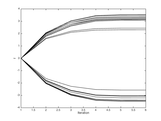
Newton-raphson procedure to optimise the latent function values

Initialise all to zero

f = repmat(0,N,1);
allf = [f'];
% Pre-compute the inverse of C
invC = inv(C);
for iteration = 2:6
    g = 1./(1+exp(-f));
    gra = t - g - invC*f;
    H = -diag(g.*(1-g)) - invC;
    f = f - inv(H)*gra;
    allf(iteration,:) = f';
end
H = -diag(g.*(1-g)) - invC;
% Plot the evolution of the f values
figure()
plot(allf,'k')
xlabel('Iteration')
ylabel('f')

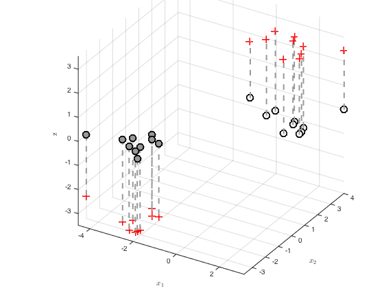
Plot the optimised latent function values

Creates a 3D plot with the function value as the z axis

figure()
hold off
pos = find(t==0);
z = zeros(length(pos),1);
plot3(x(pos,1),x(pos,2),z,'ko','markersize',10,'linewidth',2,'markerfacecolor',[0.6 0.6 0.6])
hold on
pos = find(t==1);
z = zeros(length(pos),1);
plot3(x(pos,1),x(pos,2),z,'ko','markersize',10,'linewidth',2,'markerfacecolor',[1 1 1])
for n = 1:N
    plot3(x(n,1),x(n,2),f(n),'r+','markersize',10,'linewidth',2)
    plot3([x(n,1) x(n,1)],[x(n,2),x(n,2)],[0 f(n)],'k--','color',[0.6 0.6 0.6],'linewidth',2)
end
grid on
zlabel('$f$','interpreter','latex','fontsize',20)
set(gca,'cameraviewangle',8,'cameraposition',[29.3256 -49.3194 29.7317])
set(gca,'position',[0.200 0.16 0.70 0.8150])
axis tight
xlabel('$x_1$','interpreter','latex')
ylabel('$x_2$','interpreter','latex')
zlabel('z')

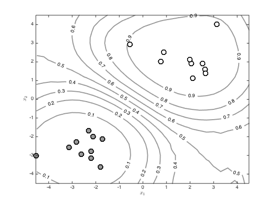
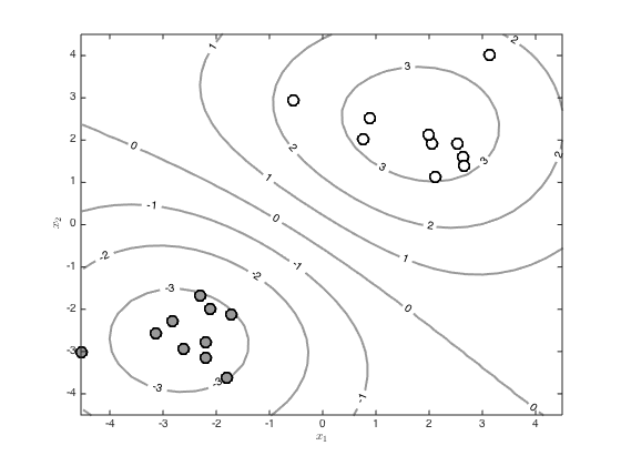
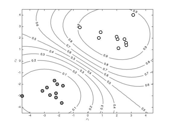
Visualise the predictive function via a large grid of test points

Create the grid

[X,Y] = meshgrid(-4.5:0.3:4.5,-4.5:0.3:4.5);
testN = prod(size(X));
testX = [reshape(X,testN,1) reshape(Y,testN,1)];
% Create the test covariance function
R = zeros(N,testN);
for n = 1:N
    for m = 1:testN
        R(n,m) = alpha*exp(-gamma*sum((x(n,:) - testX(m,:)).^2));
    end
end
% Compute the mean predictive latent function
testf = R'*invC*f;
Z = reshape(testf,size(X));
% Contour the predictions (function values, not probabilities)
figure()
hold off
[c,h]=contour(X,Y,Z,'color',[0.6 0.6 0.6]);
tl = clabel(c,h);
set(h,'linewidth',2)
hold on
pos = find(t==0);
plot(x(pos,1),x(pos,2),'ko','markersize',10,'linewidth',2,'markerfacecolor',[0.6 0.6 0.6])
pos = find(t==1);
plot(x(pos,1),x(pos,2),'ko','markersize',10,'linewidth',2,'markerfacecolor',[1 1 1])
xlabel('$x_1$','interpreter','latex')
ylabel('$x_2$','interpreter','latex')


% Contour the probabilities
figure()
hold off
[c,h]=contour(X,Y,1./(1+exp(-Z)),'color',[0.6 0.6 0.6]);
tl = clabel(c,h);
set(h,'linewidth',2)
hold on
pos = find(t==0);
plot(x(pos,1),x(pos,2),'ko','markersize',10,'linewidth',2,'markerfacecolor',[0.6 0.6 0.6])
pos = find(t==1);
plot(x(pos,1),x(pos,2),'ko','markersize',10,'linewidth',2,'markerfacecolor',[1 1 1])
xlabel('$x_1$','interpreter','latex')
ylabel('$x_2$','interpreter','latex')

Warning: Text handle output is not supported for managed labels. 
Warning: Text handle output is not supported for managed labels. 

Using the full GP distribution - propagating the uncertainity through the sigmoid

pred_var = zeros(testN,1);
pavg = zeros(size(testf));
minpred_var = 1e-3;
% loop over the test points, computing the marginal predictive variance and
% sampling function values before passing them through the sigmoid and
% averaging to get a probability

for n = 1:testN
    pred_var(n) = max(minpred_var,alpha - R(:,n)'*invC*R(:,n));
    u = randn(10000,1).*sqrt(pred_var(n)) + testf(n);
    pavg(n) = mean(1./(1+exp(-u)));
end

% Contour the resulting probabilities
Z = reshape(pavg,size(X));
figure()
hold off
[c,h]=contour(X,Y,Z,'color',[0.6 0.6 0.6]);
tl = clabel(c,h);
set(h,'linewidth',2)

hold on
pos = find(t==0);
plot(x(pos,1),x(pos,2),'ko','markersize',10,'linewidth',2,'markerfacecolor',[0.6 0.6 0.6])
pos = find(t==1);
plot(x(pos,1),x(pos,2),'ko','markersize',10,'linewidth',2,'markerfacecolor',[1 1 1])

xlabel('$x_1$','interpreter','latex')
ylabel('$x_2$','interpreter','latex')

Warning: Text handle output is not supported for managed labels. 

Published with MATLAB® R2014b