Contents
gpprior.m
Plots realisations from a GP prior using an RBF covariance function
From A First Course in Machine Learning Simon Rogers, August 2016 [simon.rogers@glasgow.ac.uk]
clear all; close all;
Define the x variable
The first step is to define the x values of interest, we'll pick some random ones in the range -5 to 5
x = rand(200,1) * 10 - 5;
x = sort(x);
Define the kernel parameters of interest
We are using an RBF covariance function:

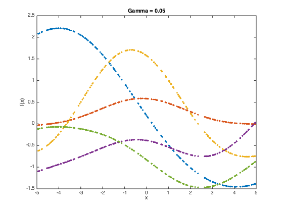
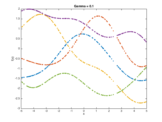
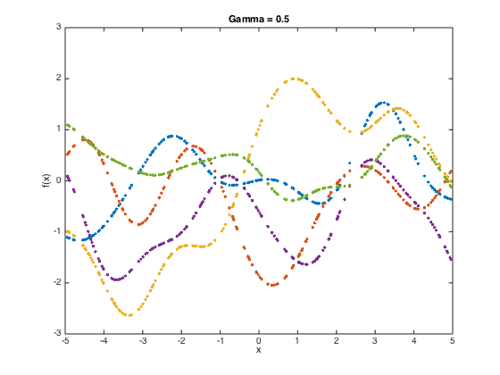
gamvals = [0.05,0.1,0.5];
alpha = 1;
Loop over the gamma values
at each stage, compute the covariance matrix and then sample 5 functions from the GP (i.e. 5 realisations from the N dimensional Gaussian with men zero and covariance equal to the covariance matrix.
N = length(x);
for gam = gamvals
    C = zeros(N);
    for n = 1:N
        for n2 = 1:N
            C(n,n2) = alpha*exp(-gam*(x(n)-x(n2))^2);
        end
    end
    % add some jitter for numerical stability
    C = C + 1e-6*eye(N);
    f = mvnrnd(repmat(0,N,1),C,5);
    figure()
    plot(x,f,'.');
    title(sprintf('Gamma = %g',gam));
    xlabel('x');
    ylabel('f(x)');
    drawnow;
end