Contents

badmh.m

Script demonstrating issues related to MH sampling when there is high correlation

From A First Course in Machine Learning Simon Rogers, August 2016 [simon.rogers@glasgow.ac.uk]

clear all; close all;

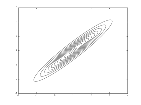
Create the Gaussian and contours for plotting

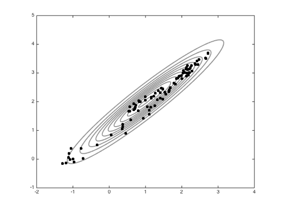
2d Gaussian with hich correlation

mu = [1;2];
co = [1 0.95;0.95 1];

[Xv,Yv] = meshgrid([-2:0.01:4],[-1:0.01:5]);

Ci = inv(co);

P = zeros(size(Xv));
for i = 1:size(Xv(:))
    P(i) = -log(2*pi)- 0.5*log(det(co)) - 0.5*([Xv(i)-mu(1) Yv(i)-mu(2)]*Ci*[Xv(i)-mu(1) Yv(i)-mu(2)]');
end
P = exp(P);
contour(Xv,Yv,P,'k','linewidth',2,'color',[0.6 0.6 0.6])

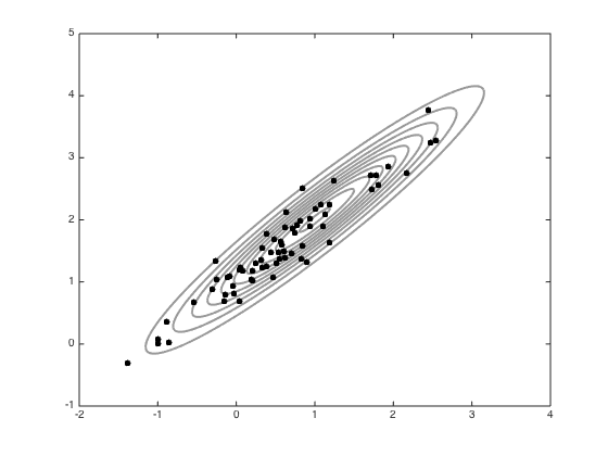
Standard MH sampling

% Define the jump variance and the number of samples
jss = 0.1;
S = 100;
all_samps = zeros(S+1,2);

% Starting point
x = [-1;0];
accept = 0;
coI = inv(co);
all_samps(1,:) = x';

% Do the sampling
for s = 1:S
    new_x = x + randn(2,1).*sqrt(jss);
    new_like = -0.5*(new_x-mu)'*coI*(new_x-mu);
    old_like = -0.5*(x-mu)'*coI*(x-mu);
    r = exp(new_like - old_like);
    if rand<r
        x = new_x;
        accept = accept+1;
    end
    all_samps(s+1,:) = x';
end


% plot the samples
n_plot = 100;
figure(1);hold off
contour(Xv,Yv,P,'k','linewidth',2,'color',[0.6 0.6 0.6])
hold on
plot(all_samps(1,1),all_samps(1,2),'ko','markersize',5,'markerfacecolor','k')
for i = 2:n_plot
    plot(all_samps(i,1),all_samps(i,2),'ko','markersize',5,'markerfacecolor','k')
end

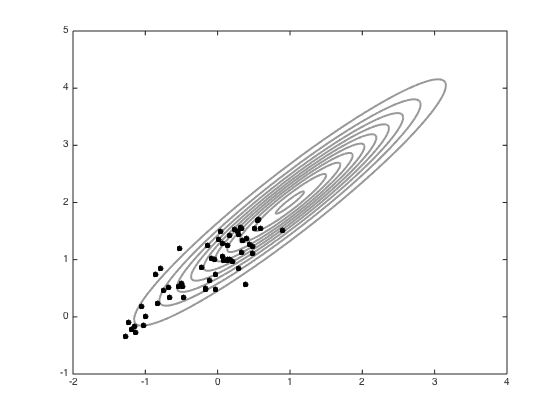
Now try adapting the proposal

Compute the sample covariance

Cs = 0.2*cov(all_samps);
figure();hold off
% Contour the gaussian and the new jump covariance
contour(Xv,Yv,P,'k','linewidth',2,'color',[0.6 0.6 0.6])
Csi = inv(Cs);
% Arbitrary mean point for the jump cov
muj = [0.5;1];
Ps = zeros(size(Xv));
for i = 1:size(Xv(:))
    Ps(i) = -log(2*pi)- 0.5*log(det(Cs)) - 0.5*([Xv(i)-muj(1) Yv(i)-muj(2)]*Csi*[Xv(i)-muj(1) Yv(i)-muj(2)]');
end
Ps = exp(Ps);
hold on
contour(Xv,Yv,Ps,'k','linewidth',2)

% Sample with this new covariance

S = 100;
all_samps_S = zeros(S+1,2);

x = [-1;0];
accept_S = 0;
coI = inv(co);
all_samps_S(1,:) = x';
for s = 1:S
    new_x = x + mvnrnd(repmat(0,2,1),Cs,1)';
    new_like = -0.5*(new_x-mu)'*coI*(new_x-mu);
    old_like = -0.5*(x-mu)'*coI*(x-mu);
    r = exp(new_like - old_like);
    if rand<r
        x = new_x;
        accept_S = accept_S + 1;
    end
    all_samps_S(s+1,:) = x';
end

% plot the samples
n_plot = 100;
figure();hold off
contour(Xv,Yv,P,'k','linewidth',2,'color',[0.6 0.6 0.6])
hold on
plot(all_samps_S(1,1),all_samps_S(1,2),'ko','markersize',5,'markerfacecolor','k')
for i = 2:n_plot
    plot(all_samps_S(i,1),all_samps_S(i,2),'ko','markersize',5,'markerfacecolor','k')
end

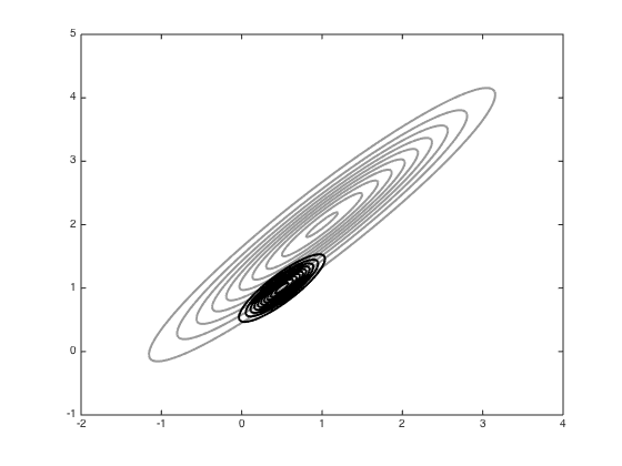
Next try Hamiltonian MCMC

Initialise parameters

M = eye(2);
iM = inv(M);
epsilon = 0.1;
L = 10;
x = [-1;0];
phi = mvnrnd(repmat(0,2,1),M,1)';
all_samps_H = zeros(S+1,2);
all_samps_H(1,:) = x';
accept_H = 0;
for s = 1:S
    new_phi = mvnrnd(repmat(0,2,1),M,1)';
    new_x = x;
    new_phi = new_phi + 0.5*epsilon*coI*(mu-new_x);
    for l = 1:L-1
        new_x = new_x + epsilon*iM*new_phi;
        new_phi = new_phi + epsilon*coI*(mu-new_x);
    end
    new_phi = new_phi + 0.5*epsilon*coI*(mu-new_x);

    new_like = -0.5*(new_x-mu)'*coI*(new_x-mu);
    old_like = -0.5*(x-mu)'*coI*(x-mu);

    new_like = new_like - 0.5*new_phi'*iM*new_phi;
    old_like = old_like - 0.5*phi'*iM*phi;

    r = exp(new_like - old_like);

    if rand<r
        x = new_x;
        accept_H = accept_H + 1;
    end
    all_samps_H(s+1,:) = x';
end

% plot the samples from HMC
n_plot = 100;
figure();hold off
contour(Xv,Yv,P,'k','linewidth',2,'color',[0.6 0.6 0.6])
hold on
plot(all_samps_H(1,1),all_samps_H(1,2),'ko','markersize',5,'markerfacecolor','k')
for i = 2:n_plot
    plot(all_samps_H(i,1),all_samps_H(i,2),'ko','markersize',5,'markerfacecolor','k')
end

Published with MATLAB® R2014b