Contents

gibbs_gp_class.m

Using gibbs sampling for binary GP classification Gaussian

From A First Course in Machine Learning Simon Rogers, August 2016 [simon.rogers@glasgow.ac.uk]

clear all;close all;

Generate a dataset

rng(222)
x = sort(rand(10,1));
N = length(x);
t = [repmat(0,5,1);repmat(1,5,1)];

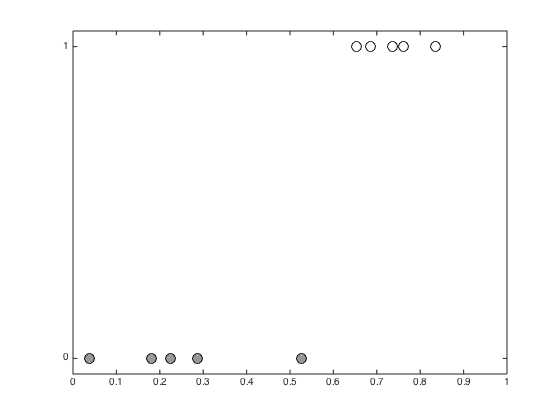
Plot the data

figure(1);hold off
pos = find(t==0);
plot(x(pos),t(pos),'ko','markerfacecolor',[0.6 0.6 0.6],'markersize',10);
hold on
pos = find(t==1);
plot(x(pos),t(pos),'ko','markerfacecolor',[1 1 1],'markersize',10);
xlim([0 1]);
ylim([-0.05 1.05]);
set(gca,'ytick',[0 1])

Define a test set for visualisation

testx = [0:0.01:1]';
Ntest = length(testx);
% Set the number of Gibbs samples to draw
S = 10000;
% Initialise the auxiliary variables, y
y = randn(size(x));
y(t==0) = y(t==0) - 2;
y(t==1) = y(t==1) + 2;

% Objects to store the sampled values
allF = zeros(S,N);
allT = zeros(S,Ntest);
allFstar = zeros(S,Ntest);
trainTall = zeros(S,N);

Set the hyperparameters and create the covariance matrices

gamma = 10.0;
alpha = 1;
C = zeros(N);
R = zeros(N,Ntest);
for n = 1:N
    for m = 1:N
        C(n,m) = alpha*exp(-gamma*(x(n)-x(m))^2);
    end
    for m = 1:Ntest
        R(n,m) = alpha*exp(-gamma*(x(n) - testx(m))^2);
    end
end

Main sampling loop

sif = inv(inv(C) + eye(N));
Ci = inv(C);
% Loop over the number of desired samples
for s = 1:S

    % Update f
    f = mvnrnd(sif*y,sif);
    allF(s,:) = f;

    % update y (using rejection sampling)
    for n = 1:N
        finished = 0;
        while ~finished
            y(n) = randn + f(n);
            if y(n)*(2*t(n)-1) > 0
                finished = 1;
            end
        end
    end

    % Sample a predictive function f^*
    f_star_mu = R'*Ci*f';
    f_star_ss = alpha - diag(R'*(C\R));

    % Look out for -ve values caused by

    f_star = randn(Ntest,1).*sqrt(f_star_ss) + f_star_mu;
    allFstar(s,:) = f_star';

    % Use this to make (and store) some predictions
    y_star = randn(Ntest,1) + f_star;
    allT(s,:) = (y_star>0)';

    tempy = randn(N,1) + f';
    trainTall(s,:) = (tempy>0)';

end

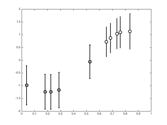
Plot the posterior f values

figure();
hold off
pos = find(t==0);
errorbar(x(pos),mean(allF(:,pos)),std(allF(:,pos)),'ko','linewidth',2,'markerfacecolor',[0.6 0.6 0.6],'markersize',10)
hold on
pos = find(t==1);
errorbar(x(pos),mean(allF(:,pos)),std(allF(:,pos)),'ko','linewidth',2,'markerfacecolor',[1 1 1],'markersize',10)
xlim([0 1])
yl = ylim;
xl = xlim;

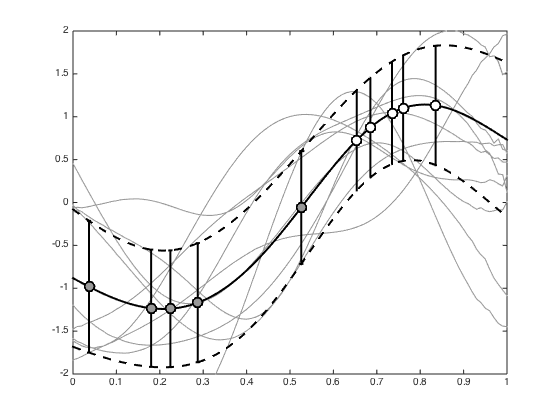
Plot 10 randomly selected samples of f from the posterior

nplot = 10;
order = randperm(S);
figure();
hold off
plot(testx,allFstar(order(1:nplot),:),'k','color',[0.6 0.6 0.6])
hold on
% Add the mean and std to the plot
plot(testx,mean(allFstar),'k','linewidth',2)
plot(testx,mean(allFstar)+std(allFstar),'k--','linewidth',2)
plot(testx,mean(allFstar)-std(allFstar),'k--','linewidth',2)
pos = find(t==0);
errorbar(x(pos),mean(allF(:,pos)),std(allF(:,pos)),'ko','linewidth',2,'markerfacecolor',[0.6 0.6 0.6],'markersize',10)
pos = find(t==1);
errorbar(x(pos),mean(allF(:,pos)),std(allF(:,pos)),'ko','linewidth',2,'markerfacecolor',[1 1 1],'markersize',10)
xlim(xl);
ylim(yl);

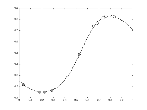
Plot the mean predictive probabilities

figure();
hold off
plot(testx,mean(allT),'k')
hold on
traint = mean(trainTall,1);
pos = find(t==0);
plot(x(pos),traint(pos),'ko','markerfacecolor',[0.6 0.6 0.6],'markersize',10);
pos = find(t==1);
plot(x(pos),traint(pos),'ko','markerfacecolor',[1 1 1],'markersize',10);

Published with MATLAB® R2014b