Contents

gibbsgauss.m

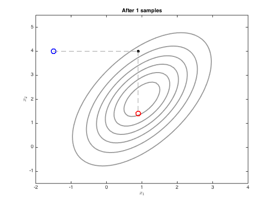
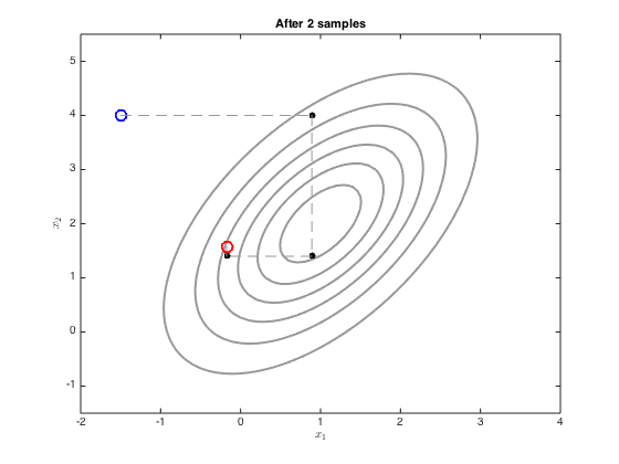
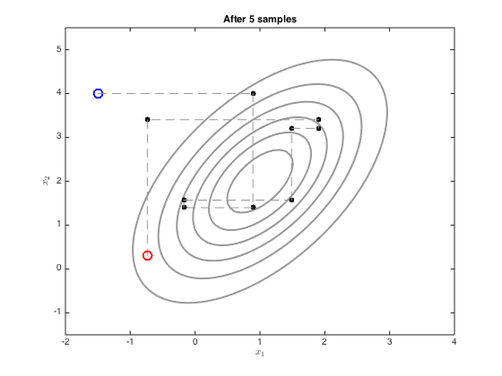
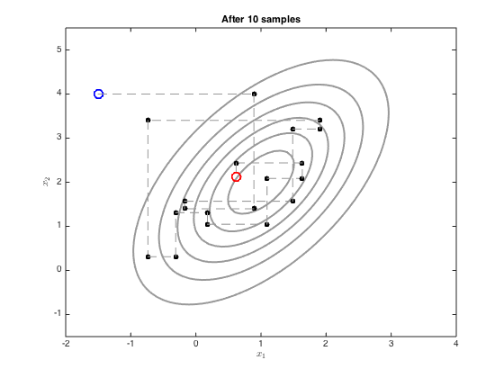
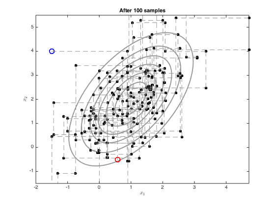
Demonstrates use of Gibbs sampling to sample from a multi-dimensional Gaussian

From A First Course in Machine Learning Simon Rogers, August 2016 [simon.rogers@glasgow.ac.uk]

clear all;close all;

First, create the objects to plot the Gaussian contour

Define the mean and covariance

mu = [1;2];
co = [1 0.8;0.8 2];
% Define a grid of points for the contours
[Xv,Yv] = meshgrid([-2:0.1:4],[-1:0.1:5]);

% Compute the pdf over the grid
Ci = inv(co);
P = zeros(size(Xv));
for i = 1:size(Xv(:))
    P(i) = -log(2*pi)- 0.5*log(det(co)) - 0.5*([Xv(i)-mu(1) Yv(i)-mu(2)]*Ci*[Xv(i)-mu(1) Yv(i)-mu(2)]');
end
P = exp(P);

We now sample with Gibbs sampling using the equations on p.317

Define the initial point - try changing this

x = [-1.5;4];
xall = x';
ylim([-1.5,5.5])

plot_at = [1,2,5,10,100];

for i = 1:100
    % Sample x_1
    mu_1 = mu(1) + (co(1,2)/co(2,2)) * (x(2)-mu(2));
    ss_1 = co(1,1) - co(1,2)^2/co(2,2);
    oldx = x;
    x(1) = randn*sqrt(ss_1) + mu_1;
    xall = [xall;x'];


    % sample x_2
    mu_2 = mu(2) + (co(2,1)/co(1,1)) * (x(1)-mu(1));
    ss_2 = co(2,2) - co(2,1)^2/co(1,1);
    oldx = x;
    x(2) = randn*sqrt(ss_2)+mu_2;

    xall = [xall;x'];

    if any(plot_at==i)
        figure(i)
        contour(Xv,Yv,P,'k','linewidth',2,'color',[0.6 0.6 0.6])
        hold on
        % Plot the initial one
        plot(xall(1,1),xall(1,2),'bo','markersize',10,'linewidth',2)
        % Plot the middle ones
        for j = 2:size(xall,1)-1
            plot([xall(j-1,1),xall(j,1)],[xall(j-1,2),xall(j,2)],'k--','color',[0.6 0.6 0.6])
            plot(xall(j,1),xall(j,2),'ko','markersize',5,'markerfacecolor','k')
        end
        % plot the end one
        plot([xall(end-1,1),xall(end,1)],[xall(end-1,2),xall(end,2)],'k--','color',[0.6 0.6 0.6])
        plot(xall(end,1),xall(end,2),'ro','markersize',10,'linewidth',2)
        ylim([-1.5,5.5])
        xlabel('$x_1$','interpreter','latex');
        ylabel('$x_2$','interpreter','latex');
        title(sprintf('After %g samples',i));
    end
end

Published with MATLAB® R2014b