Number Spirals
Introduction
The well-known Ulam spiral and the variant developed by Robert Sacks, the Sacks spiral, show interesting geometric patterns in the positions of primes. This page explores a simple extension of these spirals to visualize the number of unique prime factors for each number and provides Python code for drawing them, along with some pre-rendered examples, in PostScript and PNG format.Every image has (or should have!) the Python script used to generate it -- see the code section for details of what you need to run these. Python source code files are shown inside square brackets. You should be able to generate and play with anything you see on this page. Have fun!
Construction
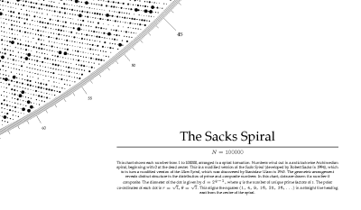
The layout of the Sacks spiral aligns the squares (1,4,9,16,... etc) along a straight line heading east from the center. Its construction is very simple: the polar co-ordinates of each integer i is just:theta = sqrt(i) * 2 * pi
r = sqrt(i),
and thus its x,y co-ordinates are given by:
x = -cos(sqrt(i)*2*pi)*sqrt(i)
y = sin(sqrt(i)*2*pi)*sqrt(i)
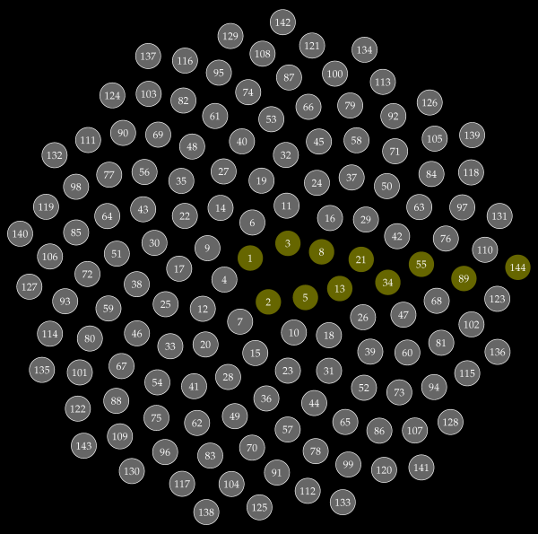
The result is a spiral like this (primes are colored bluish-green, squares olive-yellow):
Prime Factor Spirals
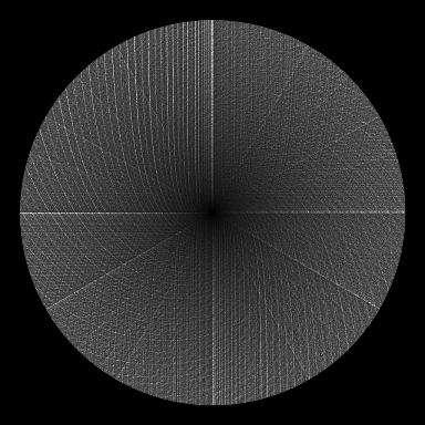
In the original construction, points are colored if they prime and uncolored if not. Dense clustering of primes along particular paths appears. This is quite unexpected, and to an extent unexplained. By generalizing to visualize the number of unique prime factors, other geometric features appear. For example, the radius of each drawn circle can be made proportional to the number of unique prime factors the associated number has. The result is an extremely rich and varied pattern.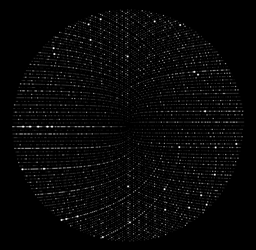
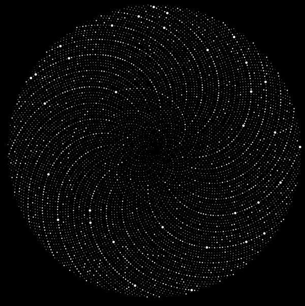
This is an image of the first 10000 numbers laid out in such a spiral, produced by the python code given below.
Why unique prime factors? Well, it seems to have a lot of visual structure -- more interesting than the same plots showing total prime factors, or other variations. It's easy to plot variations if you feel like exploring them; after all the code you need is all here.
Interesting Features -- A Short Tour
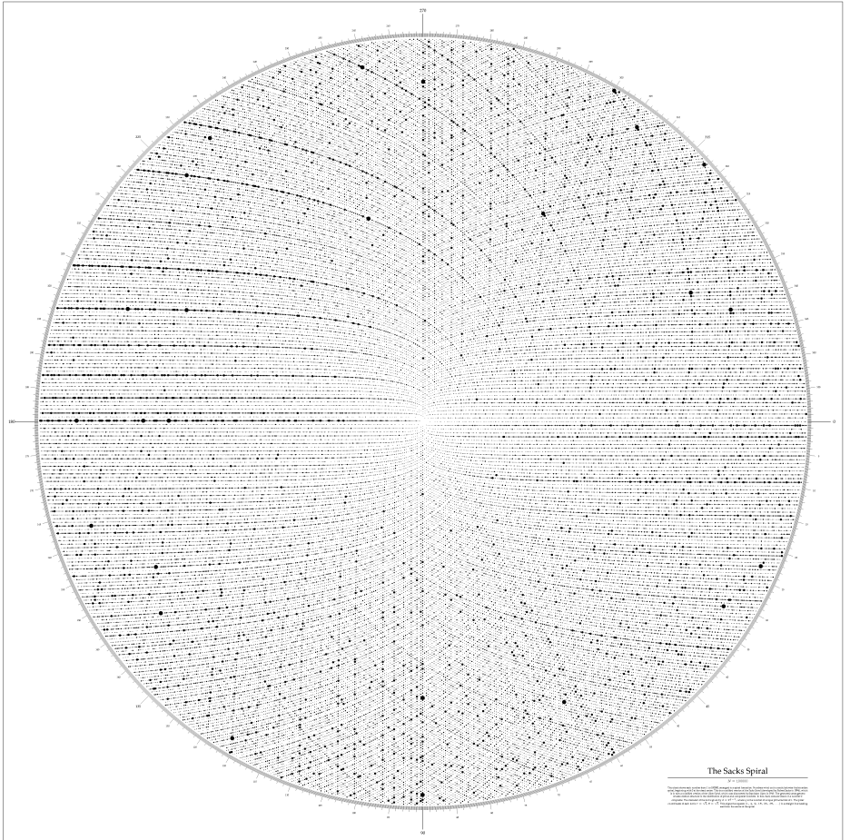
There are a number of geometric features that appear on the plots.To see most of these features, you'll need a high-resolution image of the spiral with at least 100,000 points. Either use the PostScript version spiral_1e5.ps.zip or, if you can't use that, the big PNG version . All of the angle references apply to the compass drawn around the 100,000 point version.
- The sparse curves There are several curves which are very sparse (i.e. there is a high density of prime numbers and few-factored composites). The most prominent of these meets the exterior at about 203 degrees. A second, smaller one meets the exterior at 189.5 degrees. Another meets at 37 degrees and has a fainter parallel at 29 degrees.
- The vertical lines Between about 90 and 70 degrees, and between 270 and 250, there are distinct, unevenly spaced vertical lines, getting more tightly spaced as the axes (90 and 270) are reached.
- The diagonals At exactly 60 and 300 degrees two fuzzy lines extending from the center are clearly visible. A number of fainter parallel lines can be seen, anti-clockwise from the original lines. A symmetric pair at 120 and 240 are very faintly visible.
- Dense horizontals In the quadrant from 90 to 180 degrees, numerous dense lines can be seen, becoming more tightly spaced towards 180 degrees. The line at exactly 180 degrees is the densest line on entire spiral.
Python Code
The code for generating rendering the spirals is very simple. For maximum quality, a vector format is desirable; I've used the excellent PyX package to render to PostScript.Pre-Requsites
To run these examples, you need Python, PyX (linked above), and also the elementary number theory package ent.py by William Stein. Both of these are pure Python and should run on any platform.
The simplest code looks like this (this produces the image of the first 10000 points shown earlier):
from pyx import *
from ent import *
from math import *

n = 10000
ca = canvas.canvas()

for j in range(n):
    i = j + 1
    r = sqrt(i)
    theta = r * 2 * pi
    x = cos(theta)*r
    y = -sin(theta)*r
    factors = factor(i)
    if(len(factors)>1):
        radius = 0.05*pow(2,len(factors)-1)
        ca.fill(path.circle(x,y, radius))


d = document.document(pages = [document.page(ca,
                     paperformat=document.paperformat.A4, fittosize=1)])
d.writePSfile("spiral_simple.ps")
[spiral_simple.py]
The PostScript file generated is spiral_simple.ps.zip (zipped PostScript). View it with GhostView . This could easily be changed to color the points differently instead of modulating the radius, e.g. by replacing the ca.fill() call with
ca.fill(path.circle(x,y, 0.3), color.palette.RedGreen.getcolor((len(factors)-1)/8.0)))
There are lots of visualisation techniques that could be used -- for example false coloring the image using one color channel for the number of unique factors, one for the primes, and another for the total number of factors. If you find any interesting ones, please let me know. In this code, the radius of each point is 2^(f-1) (where f is number of unique prime factors). Prime numbers are omitted entirely. The exponential scaling is largely arbitrary; I tried a number of different functions and found this to be the most revealing. Since numbers with large numbers of unique prime factors are rare in small integers (no number below 9699690 can have more than seven), the mapping works well.
Scaling Up
Unfortunately this runs out of memory fairly quickly. Since the PostScript consists of nothing but a series of arc drawing commands, this is easily (but messily) solved by splitting the PostScript file into multiple chunks and then merging them together at the end. The chunks can be topped and tailed to get rid of the header then simply slotted together. [spiral_final.py] does this.This also adds a compass (divided into tenths of degrees) around the outside of the area, and adds a textual label. NOTE: If you're using this code, you'll either need to have LaTeX installed to do the text rendering, or comment out the "texrunner" lines from the source in write_label() and draw_axis(), and live without the labels.
The output for 100,0000 points is spiral_1e5.ps.zip .
For 1,000,000 points the extremely dense result is spiral_1e6.ps.zip (WARNING: this is a 12.2MB file, and expands to 81.1 MB on decompression!)
I've renedered up to 10,000,000 points succesfully with this code. However the PostScript file is 800MB, so if you want to see you'll need to render it yourself! At this point details are extremely difficult to make out, and it takes a very long time to draw in GhostView. Printing is probably impossible except on high end printers (with >1Gb memory).
Vogel Spiral
Using Vogel's floret model for layout also gives nice results. This model gives each integer i polar co-ordinates:r = sqrt(i)
theta = i * ((2 * pi)/phi*phi),
where phi (the golden ratio) is given by:
phi = (1 + sqrt(5)) / 2.
The result of this arrangement is to align the Fibonacci numbers along the eastern axis (although the first few are slightly off axis).
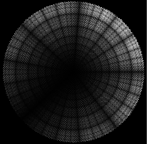
In contrast to the original spiral, which had a square on every turn, the spacing between Fibonacci numbers increases rapidly. The above image was generated by [labeled_vogel.py]. Shown below is the result for 10,000 integers. spiral_vogel_1e5.ps.zip is the 100,000 integer PostScript version. This unadorned spiral was generated with [spiral_vogel.py] .
The script [spiral_vogel_final.py] produces Vogel model spirals with legend and compass. 100,000 points version: spiral_vogel_1e5_final.ps.zip and 1,000,000 point version: spiral_vogel_1e6_final.ps.zip
The Vogel spiral has quite a different pattern when plotting the total number of factors rather than the number of unique ones (100,000 point plot). In fact, if the Vogel spiral plots of the total and unique factors are overlaid, they show very little visual relation to each other.
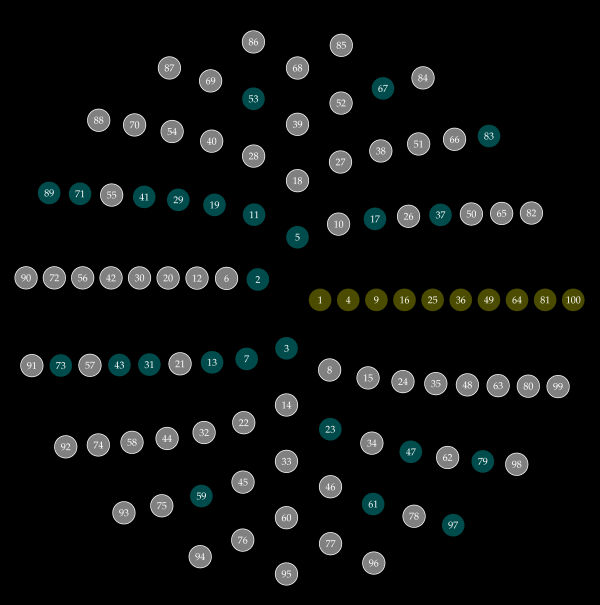
Fibonacci sums
A quick aside: every integer can be represented a sum of one or more distinct Fibonacci numbers. Some numbers cna be represented only one way (e.g. the Fibonacci numbers themselves), while others can be represented in multiple ways (e.g. 8=8, 8=5+3 and 8=5+2+1). The number of ways a number can be represented is notated H(n), and is Sloane sequence A0000119 . Plotting this function on the Vogel spiral is easy but relatively slow:
from pyx import *
from ent import *
from math import *
#fibonacci table
fibs = [0, 1, 1, 2, 3, 5, 8, 13, 21, 34, 55, 89, 144, 233, 377, 610, 987, 1597, 2584, 4181, 6765, 10946, 17711, 28657, 46368, 75025, 121393, 196418, 317811, 514229, 832040, 1346269, 2178309, 3524578, 5702887, 9227465, 14930352]
n = 10000
#recursive compute nfib(n). This is Sloane sequence A0000119
def nfib(n):
fibindex = 0
for i in fibs:
if i<=n:
fibindex = fibindex+1
fibindex -= 1
fibi = fibs[fibindex]
k = n - fibi
if n>=0 and n<=2:
return 1
elif n>2 and k>=0 and k2 and k>=fibs[fibindex-3] and k
[spiral_nfib.py]
The result is a very clear block patterning on the spiral.
PostScript version: spiral_nfib.ps.zip .
Direct Rasterization
Above 1M points, producing lossless PostScript files is too inefficient to be very useful. Instead, the points can be directly rasterized onto a grid as they are computed, and a grayscale bitmap output file created. Using a simple antialiased pixel rendering technique (Wu pixels) avoids aliasing as the image is built up. The following simple Python program does this. It uses Numeric and PIL for handling arrays and images, along with number theory package ent.py used above.
from ent import *
from math import *
import Numeric
from PIL import Image
from PIL import ImageChops
#optional: if you have psyco installed,
#uncomment these lines for a massive speed up!
#import psyco
#psyco.full()
# render a single anti-aliased pixel
def wu_pixel(surf, x, y, value):
xint = int(floor(x))
fracx = x - floor(x)
yint = int(floor(y))
fracy = y - floor(y)
btl = (1-fracx)*(1-fracy) * value
btr = (fracx)*(1-fracy) * value
bbl = (1-fracx)*(fracy) * value
bbr = (fracx)*(fracy) * value
surf[xint,yint] += btl
surf[xint+1,yint] += btr
surf[xint,yint+1] += bbl
surf[xint+1,yint+1] += bbr
#render n points on a res x res grid
def render(res, n):
#init variables
pi2 = 2*pi
half_size = res/2
basescale = (res/2.2)/ (sqrt(n)+1.0)
image = Numeric.zeros((res,res), Numeric.Float )
for j in range(n):
i = j + 1
# compute co-ordinates
r = sqrt(i)
theta = r * pi2
x = cos(theta)*r*basescale + half_size
y = -sin(theta)*r*basescale + half_size
if i%10000==0:
print '%d (%d)' %(i, int(100*i/float(n)))
#factor
factors = factor(i)
if(len(factors)>1):
strength = pow(2, len(factors)-1)
wu_pixel(image, x,y,strength)
#write the image
image = image.astype(Numeric.Int8)
mode = "L"
img = Image.fromstring(mode, (image.shape[1], image.shape[0]), image.tostring())
ImageChops.invert(img).save("spiral.png")
render(res=4096,n = 100000000)
[render.py]
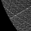
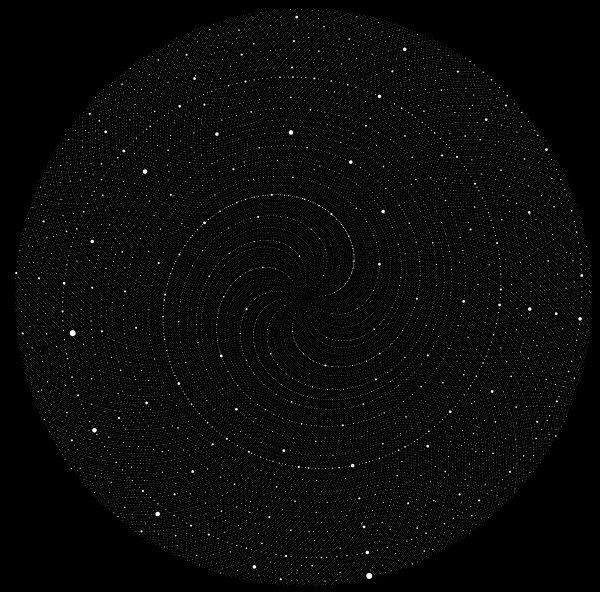
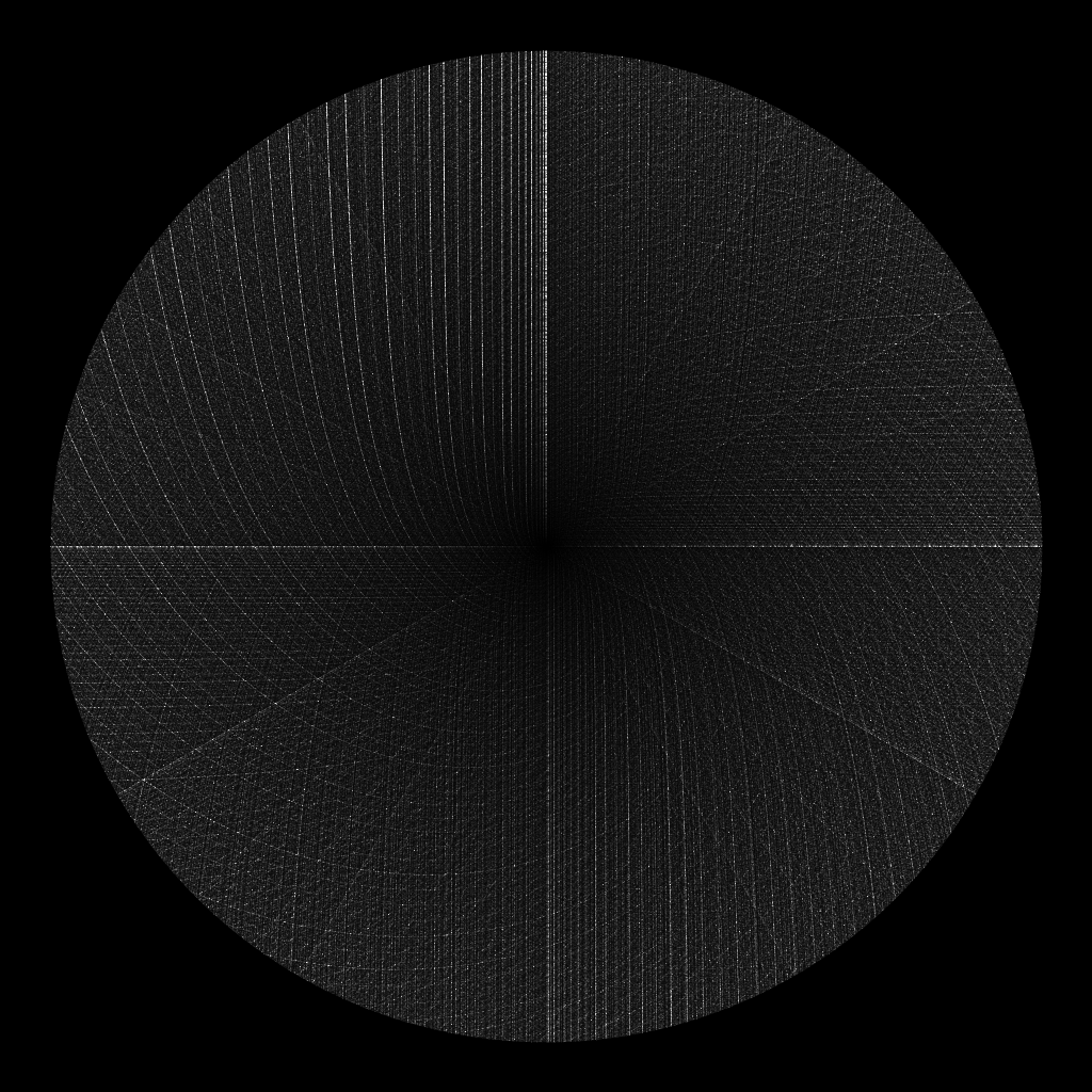
I've done renders up to 100,000,000 points with this code on a 4096 x 4096 grid. This takes about half an hour on a 3Ghz Athlon, using Psyco to speed up the python code. I am currently rendering a 1 billion point image at 8192 x 8192. The image below shows a 10,000,000 point render (click for a 1024 x 1024 version):
[render_false_color.py] renders images in false color (red = prime channel, green = unique prime factor channel, blue = total prime factor channel). In its current form, this is rather unattractive; perhaps someone else can find a nicer color visualization.
John Williamson [jhw (a/t) dcs dot gla dot ac dot uk]
